Linear Algebra Survival Kit For Data Science

Marie-Pierre Etienne

https://marieetienne.github.io/TopicsInStatistics/

2025-09-10

References on Linear Algebra for Data Scientist.

For a general overview

[Gen07]

[Har98]

[BR14]

With R or Python applications

[Yos21]

[Coh22]

Matrix computations reference book

[PP08]

Linear Algebra : What and why

Definition

Linear algebra is the branch of mathematics concerning linear equations such as \(a_1 x_1 + \cdots a_n x_n = b,\) and linear maps such as \((x_{1},\ldots ,x_{n})\mapsto a_{1}x_{1}+\cdots +a_{n}x_{n},\) and their representations in vector spaces and through matrices.

Data are organized in rectangular array, understood as matrices, and the mathematical concept associated with matrices are used to manipulate data.

Palmer penguins illustration

## install.packages('palmerpenguins")
library("palmerpenguins")
penguins_nona <- na.omit(penguins) ## remove_na for now
penguins_nona |> print(n=3)
# A tibble: 333 × 8
  species island    bill_length_mm bill_depth_mm flipper_length_mm body_mass_g
  <fct>   <fct>              <dbl>         <dbl>             <int>       <int>
1 Adelie  Torgersen           39.1          18.7               181        3750
2 Adelie  Torgersen           39.5          17.4               186        3800
3 Adelie  Torgersen           40.3          18                 195        3250
# ℹ 330 more rows
# ℹ 2 more variables: sex <fct>, year <int>
  • One row describes one specific penguin,
  • One column corresponds to one specific attribute of the penguin.

Focusing on quantitative variables, we get rectangular array with n=333 rows, and d=5 columns.

Each penguin might be seen as a vector in \(\mathbb{R}^d\) and each variable might be seen as a vector in \(\mathbb{R}^n\). The whole data set is a matrix of dimension \((n,d)\).

Linear Algebra : What and why

Regression Analysis

  • to predict one variable, the response variable named \(Y\), given the others, the regressors

  • or equivalently to identify a linear combination of the regressors which provide a good approximation of the responsbe variable,

  • or equivalently to specify parameters \(\theta,\) so that the prediction \(\hat{Y} = X \theta,\) linear combination of the regressors which is as close as possible from \(Y\).

We are dealing with linear equations, enter the world of Linear Algebra.

Principal Component Analysis

  • to explore relationship between variables,

  • or equivalently to quantify proximity between vectors,

  • but also to define a small set of new variables (vectors) which represent most of the initial variables,

We are dealing with vectors, vector basis, enter the world of Linear Algebra.

Linear Algebra Basic objects

Vectors

\(x\in \R^n\) is a vector of \(n\) components.

By convention, \(x\) is a column vector \[x=\begin{pmatrix} x_1 \cr \vdots\cr x_n \end{pmatrix}.\]

When a row vector is needed we use operator \(\ ^\intercal,\)

\[x^\intercal = \begin{pmatrix} x_1, \cdots, x_n \end{pmatrix}.\] The null vector \(\mathbb{0}\in\R^d\),

\[\mathbb{0}^\intercal = \begin{pmatrix} 0, \cdots 0\end{pmatrix}.\]

Matrix

A matrix \(A\in \R^{n\times d}\) has \(n\) rows and \(d\) columns:

\[A = \begin{pmatrix} a_{11} & a_{12} & \cdots & a_{1d} \cr a_{21} & a_{22} & \cdots & a_{2d} \cr \vdots & \vdots & & \vdots \cr a_{n1} & a_{n2} & \cdots & a_{nd} \end{pmatrix}\]

The term on row \(i\) and column \(j\) is refered to as \(a_{ij}\),

The column \(j\) is refer to as \(A_{.,j}\), \(A_{.,j} = \begin{pmatrix} a_{1j} \cr \vdots\cr a_{nj} \end{pmatrix}.\)

To respect the column vector convention, the row \(i\) is refer to as \(A_{i,.}^\intercal\), \(A_{i,.}^\intercal = \begin{pmatrix} a_{i1}, & \cdots & , a_{id} \end{pmatrix}\)

Basic operations

Simple operations

Multiplication by a scalar

let’s \(\lambda\in\R\),

\[\lambda x = \begin{pmatrix} \lambda x_1 \cr \vdots\cr \lambda x_n \end{pmatrix}.\]

\[\lambda A = \begin{pmatrix} \lambda a_{11} & \lambda a_{12} & \cdots & \lambda a_{1d} \cr \lambda a_{21} & \lambda a_{22} & \cdots & \lambda a_{2d} \cr \vdots & \vdots & & \vdots \cr \lambda a_{n1} & \lambda a_{n2} & \cdots & \lambda a_{nd} \end{pmatrix}\]

Sum

If \(x\in \R^n\) and \(y\in R^n\), then \(x+y\) exists

\[x+ y = \begin{pmatrix} x_1 + y_1 \cr \vdots\cr x_n + y_n\end{pmatrix}.\]

If \(A\) and \(B\) are two matrices with the same dimensions, \(A+B\) exists

\[ A+B = \begin{pmatrix} a_{11} + b_{11} & \cdots & a_{1d} + b_{1d}\cr \vdots & & \vdots \cr a_{n1} + b_{n1}& \cdots & a_{nd} + b_{nd} \end{pmatrix}. \]

Visualization

Consider \(x=\begin{pmatrix} 1 \cr 0 \end{pmatrix}\) and \(y= \begin{pmatrix} 0 \cr 1 \end{pmatrix},\) and \(z=x+2 y.\)

Matrix product

Let \(A\in \R^{n \times p}\) and \(B\in\R^{p \times d}\), then the product \(AB\) is well defined, it is a matrix \(C\) in \(\R^{n\times ,d}\), so that

\[C_{ij} = \sum_{k=1}^p A_{ik} B_{kj}, \quad 1\leq i\leq n, 1\leq j \leq d.\]

Example

  • \(A\in \R^{3 \times 2}\), \(B\in\R^{2 \times 4}\), with \(A = \begin{pmatrix} \color{color }{1} & 2 \cr 1 & 3 \cr -1 & -1 \end{pmatrix}\) and \(B =\begin{pmatrix} {-1} & {-2} & {0} & {1}\cr {-2} & {1} & {1} & {0}\end{pmatrix},\)

\(A B\) exists as the number of colums in \(A\) equals the number of rows in \(B\).

A useful presentation: \[\begin{matrix} & & \begin{pmatrix} \class{bleuf}{-1} & \class{bleu}{-2} & \class{vert}{0} & \class{clair}{1}\cr \class{bleuf}{-2} & \class{bleu}{1} & \class{vert}{1} & \class{clair}{0}\end{pmatrix} \cr & \begin{pmatrix} \class{jaune}{1} & \class{jaune}{2} \cr \class{orange}{1} & \class{orange}{3} \cr \class{rouge}{-1} & \class{rouge}{-1} \end{pmatrix} & \begin{pmatrix} \class{jaune}{\bullet} \class{bleuf}{\bullet} & \class{jaune}{\bullet} \class{bleu}{\bullet} & \class{jaune}{\bullet} \class{vert}{\bullet} & \class{jaune}{\bullet} \class{clair}{\bullet} \cr \class{orange}{\bullet} \class{bleuf}{\bullet} & \class{orange}{\bullet} \class{bleu}{\bullet} & \class{orange}{\bullet} \class{vert}{\bullet} & \class{orange}{\bullet} \class{clair}{\bullet} \cr \class{rouge}{\bullet} \class{bleuf}{\bullet} & \class{rouge}{\bullet} \class{bleu}{\bullet} & \class{rouge}{\bullet} \class{vert}{\bullet} & \class{rouge}{\bullet} \class{clair}{\bullet} \cr \end{pmatrix}, \end{matrix} \] * \[AB = \begin{pmatrix} \class{jaune}{1}\times\class{bleuf}{(-1)} +\class{jaune}{2}\times \class{bleuf}{(-2)} & \class{jaune}{1}\times \class{bleu}{(-2)} + \class{jaune}{2} \times\class{bleu}{1} & \class{jaune}{1}\times \class{vert}{0} + \class{jaune}{2}\times \class{vert}{1} & \class{jaune}{1} \times\class{clair}{1} + \class{jaune}{2}\times \class{clair}{0} \cr \class{orange}{1} \times \class{bleuf}{(-1)} + \class{orange}{3} \times \class{bleuf}{(-2)} & \class{orange}{1} \times \class{bleu}{(-2)} + \class{orange}{3} \times \class{bleu}{1} & \class{orange}{1} \times \class{vert}{0} + \class{orange}{3} \times \class{vert}{1} & \class{orange}{1} \times\class{clair}{1} + \class{orange}{3}\times \class{clair}{0} \cr \class{rouge}{(-1)} \times \class{bleuf}{(-1)} + \class{rouge}{(-1)} \times \class{bleuf}{(-2)} & \class{rouge}{(-1)} \times \class{bleu}{(-2)} + \class{rouge}{(-1)} \times \class{bleu}{1} & \class{rouge}{(-1)} \times \class{vert}{0} + \class{rouge}{(-1)} \times \class{vert}{1} & \class{rouge}{(-1)} \times\class{clair}{1} + \class{rouge}{(-1)}\times \class{clair}{0} \cr \end{pmatrix},\]

\[AB = \begin{pmatrix} -5 & 0 & 2 & 1 \cr -7 & 1 & 3 & 1 \cr 3 & 1 &-1 & -1 \cr \end{pmatrix}. \]

A matrix is defined column by column

A = matrix(c(1,1,-1,2,3,-1), ncol = 2)
B = matrix(c(-1,-2, -2,1, 0, 1, 1, 0), ncol = 4)

The default operation \(A*B\) is not the matrix product but a product element by element, the matrix product is obtained by

A %*% B
     [,1] [,2] [,3] [,4]
[1,]   -5    0    2    1
[2,]   -7    1    3    1
[3,]    3    1   -1   -1

Matrix product is available through the numpy library

import numpy as np

A = np.array([[ 1, 2], [ 1, 3], [ -1, 1]]); A.view()
array([[ 1,  2],
       [ 1,  3],
       [-1,  1]])
B = np.array([[-1, -2, 0, 1], [ -2, 1, 1, 0]]); B.view()
array([[-1, -2,  0,  1],
       [-2,  1,  1,  0]])
C = A.dot(B);  C.view()
array([[-5,  0,  2,  1],
       [-7,  1,  3,  1],
       [-1,  3,  1, -1]])

Matrix vector product

As a vector \(x\) in \(\R^n\) is also a matrix in \(\R^{n\times 1}\), the product \(A x\) exisst is the number of columns in \(A\) equals the number of row for \(x\).

\[A = \begin{pmatrix} 1 & -1 \cr 1 & 0 \cr -1 & 0.5 \end{pmatrix},\]

Let \(x\in \R^2\), \(Ax\) exists

\[Ax = \begin{pmatrix} x_1 - x_2 \cr x_1 \cr -x_1 + 0.5 x \end{pmatrix},\]

Let \(x\in\R^2\), \(y\in\R^3\) and \[A = \begin{pmatrix} 1 & -1 & 0 \cr 1 & 0 & -0.5 \cr -1 & 0.5 & 2 \end{pmatrix}, B = \begin{pmatrix} 1 & 1 & 0 \cr -1 & 0 & -0.5 \end{pmatrix},\quad C = \begin{pmatrix} 1 & -1 \cr -1 & 2 \cr 1 & -0.5 \end{pmatrix},\]

When possible, compute the following quantites

\[ Ax; \quad Ay; \quad AB; \quad BA; \quad AC; \quad CA; \quad Bx; \quad Cx. \]

Transposition

The transpose, denoted by \(\ ^\intercal\), of a matrix results from switching the rows and columns. Let \(A \in \R^{n\times d}\), \[A^{\intercal} \in \R^{d\times n},\ and (A^{\intercal})_{ij}= A_{ji}.\]

\[ A = \begin{pmatrix} \class{jaune}{\bullet} & \class{jaune}{\bullet} \cr \class{orange}{\bullet} & \class{orange}{\bullet} \cr \class{rouge}{\bullet} & \class{rouge}{\bullet} \cr \end{pmatrix}, \quad A^{\intercal} = \begin{pmatrix} \class{jaune}{\bullet} & \class{orange}{\bullet} & \class{rouge}{\bullet}\cr \class{jaune}{\bullet} & \class{orange}{\bullet} & \class{rouge}{\bullet} \end{pmatrix} \]

Example

\[A = \begin{pmatrix} 1 & -1 \cr 1 & 0 \cr -1 & 0.5 \end{pmatrix}, \quad A^\intercal = \begin{pmatrix} 1 & 1 & -1 \cr -1 & 0 & 0.5 \end{pmatrix}, \]

Properties

  • \((A^\intercal)^\intercal = A,\)
  • \((AB)^\intercal = (B)^\intercal (A)^\intercal,\)
  • \((A+B)^\intercal = (A)^\intercal + (B)^\intercal.\)

\[A = \begin{pmatrix} 1 & -1 & 0 \cr 1 & 0 & -0.5 \cr -1 & 0.5 & 2 \end{pmatrix}, B = \begin{pmatrix} 1 & 1 & 0 \cr -1 & 0 & -0.5 \end{pmatrix}, C=\begin{pmatrix} 1 & 2 \cr 2 & 1 \end{pmatrix}, x \in \R^2, y\in\R^3.\]

Compute \((C)^\intercal, (BA)^\intercal, x^\intercal B, (Ay)^\intercal, y^\intercal A^\intercal\)

Dot product and norm

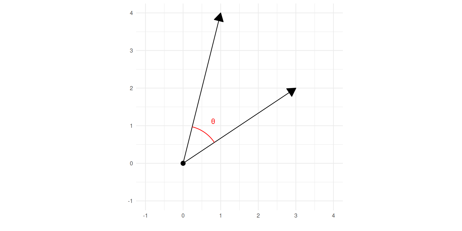
Let \(x,y\) be in \((\R^n)^2,\) the dot product, also known as inner product or scalar product is defined as \[x\cdot y = y\cdot x = \sum_{i=1}^n x_i y_i = x^\intercal y= y^\intercal x.\] The norm of a vector \(x\), symbolized with \(\norm{x},\) is defined by \[\norm{x}^2 =\sum_{i=1}^n x_i^2 = x^\intercal x.\]

\[x=\begin{pmatrix} 1\cr 0 \end{pmatrix}, y=\begin{pmatrix} 0\cr 1 \end{pmatrix}, z=\begin{pmatrix} 1\cr 2 \end{pmatrix} \]

\[x\cdot y = 0, x\cdot z = 1, y \cdot z = 2, \quad \norm{x}=\norm{y}=1, \quad \norm{z} = \sqrt{5}\]

Let \((x,y)\in(\R^n)^2\),

\(x\cdot y = \norm{x} \norm{y} \cos(\theta)\)

\(\cos(\theta)= \frac{x\cdot y}{\norm{x} \norm{y}}\)

Linear independance

A sequence of vectors \(x_1, \cdots, x_k\) from \(\R^n\) is said to be linearly independent, if the only solution to \(\sum_{i=1}^k a_i x_i =\mathbb{0}\) is \(a =\mathbb {0}\).

\(x_1 = \begin{pmatrix} 1 \cr 0 \cr 0 \end{pmatrix}, \quad x_2 = \begin{pmatrix} 1 \cr 1 \cr 0 \end{pmatrix}, \quad X=\begin{pmatrix} 1 & 1 \cr 0 & 1 \cr 0 & 0 \cr \end{pmatrix}, \quad Xa = \begin{pmatrix}a_1 + a_2\cr a_2 \cr 0 \end{pmatrix}.\)

\(x_1\) and \(x_2\) are linearly independant.

\(x_1 = \begin{pmatrix} 1 \cr 1 \cr 1 \end{pmatrix}, \quad x_2 = \begin{pmatrix} 1 \cr 1 \cr 0 \end{pmatrix}, x_3 = \begin{pmatrix} 0 \cr 1 \cr 1 \end{pmatrix}, x_4 = \begin{pmatrix} 0 \cr -1 \cr 1 \end{pmatrix}\)

  • Are \((x_1, x_2,x_3)\) linearly independant ?
  • Are \((x_1, x_2,x_4)\) linearly independant ?

Span of a set of vectors

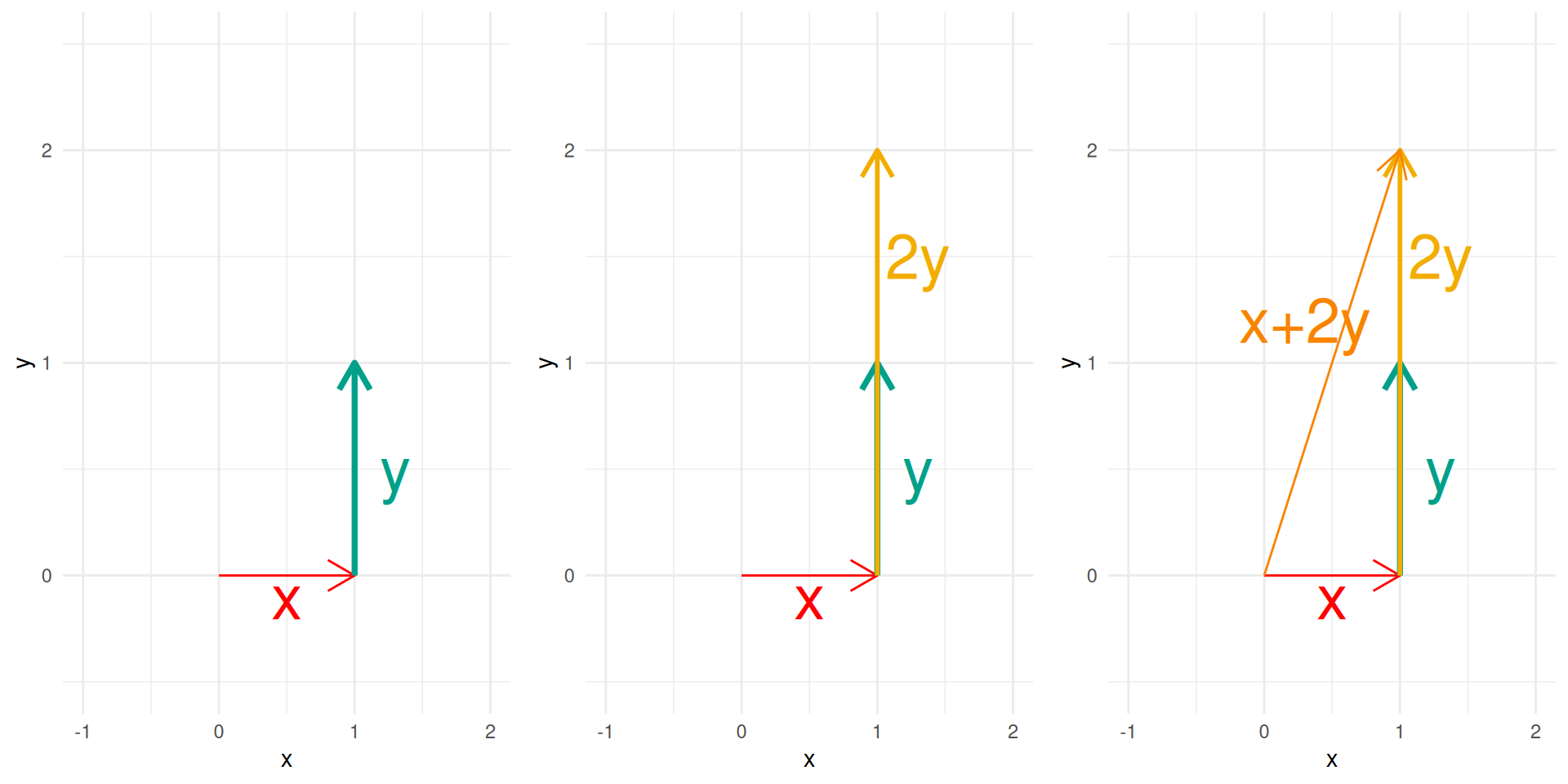
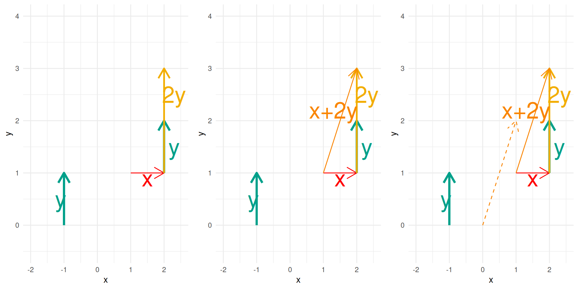
The span of a set of vectors is the set of all possible linear combinations of these vectors.
In other words, if you take some vectors \(v_1, v_2, \dots, v_k\), their span is the collection of vectors you can build by multiplying each \(v_i\) by a scalar and then adding the results together.

Formally:

\[ \text{span}(v_1, v_2, \dots, v_k) = \{ a_1 v_1 + a_2 v_2 + \cdots + a_k v_k \;\mid\; a_1, a_2, \dots, a_k \in \mathbb{R} \}. \]

Intuitively, the span represents the space generated by those vectors:

  • If you have a single nonzero vector in \(\mathbb{R}^2\), its span is a line through the origin.
  • If you have two linearly independent vectors in \(\mathbb{R}^2\), their span is the whole plane.
  • In higher dimensions, the span gives you the smallest subspace that contains all the vectors.

\[\text{span}\left(\begin{pmatrix} 1 \\ 0 \end{pmatrix}, \begin{pmatrix} 0 \\ 1 \end{pmatrix}\right );\] \[\text{span}\left(\begin{pmatrix} 1 \\ 1 \end{pmatrix}, \begin{pmatrix} 0 \\ 1 \end{pmatrix}\right );\] \[\text{span}\left(\begin{pmatrix} 1 \\ 1 \\1\end{pmatrix}, \begin{pmatrix} 0 \\ 1 \\ 1 \end{pmatrix}, \begin{pmatrix} 1 \\ 0 \\ 0 \end{pmatrix}\right );\]

Vector space

Definition

A real vector space \((V, +, . ,\R)\) is a set \(V\) equipped with two operations satisfybing the following properties for all \((x,y,z)\in V^3\) and all \((\lambda,\mu)\in\R^2:\)

  • (close for addition) \(x + y \in V,\)
  • (close for scalar multiplication) \(\lambda x \in V,\)
  • (commutativity) \(x + y = y + x,\)
  • (associativity of +) \((x + y) + z = x + (y + z),\)
  • (Null element for +) \(x + \mathbb{0} = x,\)
  • (Existence of additive inverse +) There exists \(-x \in V\), such that $ + (-x) = ,$
  • (Associativity of scalar multiplication) \(\lambda (\mu x) = (\lambda \mu ) x,\)
  • (Distributivity of scalar sums) \((\lambda + \mu ) x = \lambda x + \mu x,\)
  • (Distributivity of vector sums) \(\lambda (x + y ) = \lambda x + \lambda y,\)
  • (Scalar multiplication identity) \(1 x = x.\)

It is enough for the course to think to the set of vectors in \(\R^d\).

Basis of a Vector Space

A set B of elements of a vector space V is called a basis if every element of V can be written in a unique way as a finite linear combination of elements of B.

A subset \(B \subset V\) is a basis if it satisfies the two following conditions:

  1. Linear independence. For every finite subset \(\{ \mathbf{v}_1, \dotsc, \mathbf{v}_m \}\) of \(B\),
    if \[ c_{1}\mathbf{v}_{1} + \cdots + c_{m}\mathbf{v}_{m} = \mathbf{0} \Longleftrightarrow c_{1} = \cdots = c_{m} = 0. \]

  2. Spanning property. For every \(\mathbf{v} \in V\), there exits \(a_{1}, \dotsc, a_{n} \in \R\) such that \[ \mathbf{v} = a_{1}\mathbf{v}_{1} + \cdots + a_{n}\mathbf{v}_{n}. \]

The coefficients of this linear combination are referred to as components or coordinates of the vector with respect to B. The elements of a basis are called basis vectors.

If \(\norm{v_i} =1\) for all \(i\), the basis is orthonormal.

\(\left (\begin{pmatrix} 1 \\ 0 \end{pmatrix}, \begin{pmatrix} 0 \\ 1 \end{pmatrix}\right )\) is a basis of \(\R^2\)

Check whether or not these sets of vectors form orthobormal bases

  • in \(\R^2\) \(\left(\begin{pmatrix} 2 \\ 0 \end{pmatrix}, \begin{pmatrix} -1 \\ 2 \end{pmatrix}\right )\)

  • in \(\R^2\) \(\left(\begin{pmatrix} \sqrt{2}/2 \\ \sqrt{2}/2 \end{pmatrix}, \begin{pmatrix} -\sqrt{2}/2 \\ \sqrt{2}/2 \end{pmatrix}\right )\)

  • in \(\R^3\) \(\left(\begin{pmatrix} \sqrt{2}/2 \\ \sqrt{2}/2 \\ 1\end{pmatrix}, \begin{pmatrix} -\sqrt{2}/2 \\ 1\\ \sqrt{2}/2 \end{pmatrix}\right )\)

  • in \(\R^3\) \[{v}_1=\frac{1}{\sqrt{3}}\begin{pmatrix}1\\1\\1\end{pmatrix},\qquad v_2=\frac{1}{\sqrt{2}}\begin{pmatrix}1\\-1\\0\end{pmatrix},\qquad {v}_3=\frac{1}{\sqrt{6}}\begin{pmatrix}1\\1\\-2\end{pmatrix}.\]

Linear mapping

Let \(f\) be a function from \(\R^d\) to \(\R^n\), \(f\) is linear if and only if

For all \((\lambda,\mu) \in \R^2\) and for all \((x,y) (\R^d)^2,\) \[f(\lambda x + \mu y ) = \lambda f(x) + \mu f( y )\]

Example

\[\begin{align} f : \R^2 & \to \R\cr x & \mapsto x_1-x_2 \end{align}\]

\[\begin{align} f(\lambda x + \mu y) & = f \left ( \begin{pmatrix} \lambda x_1 + \mu y_1\cr \lambda x_2 + \mu y_2\cr \end{pmatrix} \right) = (\lambda x_1 + \mu y_1) - (\lambda x_2 + \mu y_2)=\lambda (x_1 - x_2) + \mu (y_1 -y_2)\cr & = \lambda f( x ) + \mu f( y )\cr \end{align}\]

\[f(x) = A x, \quad A = \begin{pmatrix} 1 & -1 \end{pmatrix}\]

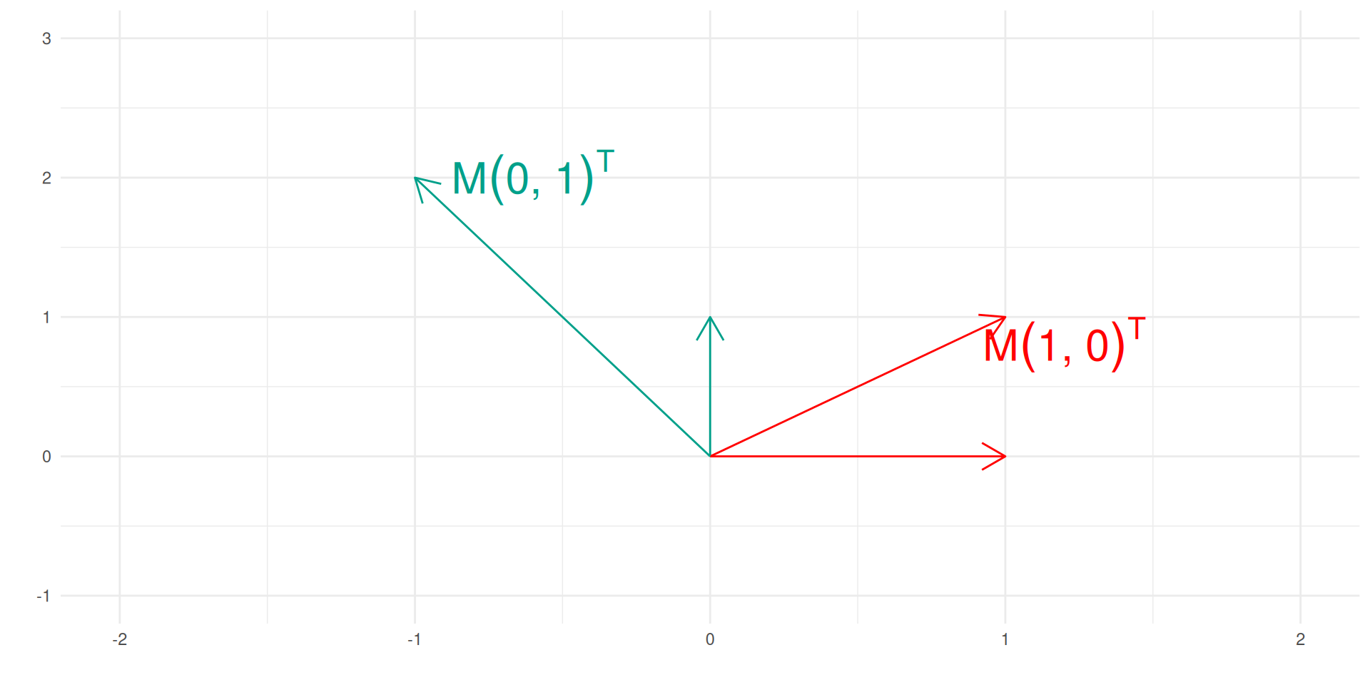
Matrix as a linear map on vector space

A real matrix \(A\in\R^{n\times d}\) is a linear function operating from one real vector space of dimension \(d\) to real vector space of dimension \(n\).

\[\begin{align} A: &\R^d \to \R^n\\ & x \mapsto y = Ax \end{align}\]

\[A = \begin{pmatrix} \color{color }{1} & 2 \cr 1 & 3 \cr -1 & -1 \end{pmatrix}\]

\[\begin{align} A: &\R^2 \to \R^3\\ & x \mapsto y = \begin{pmatrix} \color{color }{1} & 2 \cr 1 & 3 \cr -1 & -1 \end{pmatrix} \begin{pmatrix} x_1\cr x_2 \end{pmatrix} =\begin{pmatrix} x_1 + 2 x_2 \cr x_1 + 3 x_2 \cr -x_1-x_2 \end{pmatrix} \end{align}\]

\[M = \begin{pmatrix} \color{color }{1} & -1 \cr 1 & 2 \end{pmatrix}\]

\[\begin{align} & x \mapsto y = \begin{pmatrix} 1 & -1 \cr 1 & 2 \end{pmatrix} \begin{pmatrix} x_1\cr x_2 \end{pmatrix} =\begin{pmatrix} x_1 - x_2 \cr x_1 + 2 x_2 \end{pmatrix} \end{align}\]

\(A \begin{pmatrix}1\cr 0\end{pmatrix} = A_{.,1}\)

\(A \begin{pmatrix} 0\cr 1\end{pmatrix} = A_{.,2}.\)

\[\begin{align} M: &\R^2 \to \R^2\\ & x \mapsto y = \begin{pmatrix} 1 & -1 \cr 1 & 2 \end{pmatrix} x \end{align}\] is a transformation of \(\R^2\)

Exercice 1

Let’s consider the application from \(\R^2\) to \(\R^2\) which projects on the \(x\) axis.

  • Is it a linear transformation of \(\R^2\) ?
  • If so, could you write the corresponding matrix \(P\) ?

Exercice 2

Let’s consider the application from \(\R^2\) to \(\R\) which computes the square norm of the vector \(|| x||^2 = x_1^2 + x_2^2\)

  • Is it a linear transformation of \(\R^2\) ?
  • If so, could you write the corresponding matrix \(N\) ?

Exercice 1

  • Projection on \(x\) axis consists in forgetting the \(y\) axis component. \[\begin{align} f(\lambda_1 x + \lambda_2 z) & = f\left ( \begin{pmatrix} \lambda_1 x_1 + \lambda_2 z_1 \cr \lambda_1 x_1 + \lambda_2 z_2\cr \end{pmatrix} \right) \cr & = \begin{pmatrix} \lambda_1 x_1 + \lambda_2 z_1 \cr 0\cr \end{pmatrix}\cr & = \lambda_1 f(x) + \lambda_2 f(z), \end{align}\]

  • \(f\) is linear, its matrix form \(P:\)

\[P = \begin{pmatrix} 1 & 0 \cr 0 & 0 \end{pmatrix},\]

\[Px = \begin{pmatrix} 1 & 0 \cr 0 & 0 \end{pmatrix} \begin{pmatrix} x_1 \cr x_2 \end{pmatrix} = \begin{pmatrix} x_1 \cr 0 \end{pmatrix}\]

Exercice 2

  • Square Norm \(f\) of \(x\) equals \(x_1^2 + x_2^2,\) As \(f(\lambda_1 x ) = \lambda_1^2 f( x)\), the square norm is not a linear function and could not be expressed as a matrix.

Matrix rank

The sequence of columns of a matrix \(M\in \R^{n\times d}\) forms a sequence of \(d\) vectors \((c_1, \cdots,c_d)\) in \(\R^n\), while the rows of a matrix forms a sequence of \(n\) vectors \((r_1, \cdots,r_n)\) in \(\R^d\).

The rank of a matrix is the length of the largest sequence of linearly independent columns or equivalently the length of the largest sequence of linearly independent rows.

  • \(X_1 =\begin{pmatrix} 1 & 1 \cr 0 & 1 \cr 0 & 0 \cr \end{pmatrix}, \quad rank(X_1) = 2; \quad \quad X_2=\begin{pmatrix} 1 & 1 & 0 \cr 1 & 1 & -1\cr 1 & 0 & 1 \end{pmatrix}, \quad rank(X_2) = 3;\)
  • \(X_3=\begin{pmatrix} 1 & 1 & -1 \cr 1 & 1 & -1\cr 1 & 0 & 1 \end{pmatrix}, \quad rank(X_3) = 2;\)

Let \(A= (a_1, \cdots, a_d)^\intercal \in \R^d\), \(A A^\intercal = \begin{pmatrix} & & \cr a_1 A & \cdots & a_d A\cr & & \cr \end{pmatrix}\) if of rank \(1\).

#install.packages('Matrix')
library(Matrix)
X1 <- matrix(c(1,0,0,1,1,0), ncol = 2)
X2 <- matrix(c(1,1,1,1,1,0, 0, -1,1), ncol = 3)
X3 <- matrix(c(1,1,1,1,1,0, -1, -1,1), ncol = 3)
rankMatrix(X1)[1]
[1] 2
rankMatrix(X2)[1]
[1] 3
rankMatrix(X3)[1]
[1] 2
import numpy as np
from numpy.linalg import matrix_rank

X1 = np.array([[ 1, 1], [ 0, 1], [ 0, 0]])
X2 = np.array([[ 1, 1, 0], [ 1, 1, -1], [ 1, 0, 1]])
X3 = np.array([[ 1, 1, -1], [ 1, 1, -1], [ 1, 0, 1]])

matrix_rank(X1) 
np.int64(2)
matrix_rank(X2) 
np.int64(3)
matrix_rank(X3) 
np.int64(2)

Column Space, rank

If \(A\in\R^{n\times d},\) and \(c\in \R^d\), \[A c = \begin{pmatrix} & & & \cr A_{.,1} & A_{.,2} & \cdots & A_{.,d} \cr & & & \cr \end{pmatrix} \begin{pmatrix} c_1 \cr c_2 \cr \vdots \cr c_d \cr \end{pmatrix} = \begin{pmatrix} c_1 a_{11} + c_2 a_{12} + \cdots + c_d a_{1d} \cr \vdots \cr c_1 a_{n1} + c_2 a_{n2} + \cdots + c_d a_{nd} \cr \end{pmatrix} = c_1 A_{.,1} + c_2 A_{.,2} + \cdots + c_d A_{.,d}\]

Image of \(A\) or Column space of A

\(Im(A) = \left \lbrace y \in \R^d; \exists c\in R^d, y = \sum_{l=1}^d c_l A_{., l} \right \rbrace\)

Remarks

  • If \(A_{.,1}\) and \(A_{,2}\) are linearly dependant, \(A_{,1} = \lambda A_{,2}\) and \(Ac = ( c_1 \lambda + c_2) A_{.,2} + \cdots + c_d A_{.,d}\). The rank is the minimal number of vector to generate \(Im(A)\), that is the dimension of \(Im(A)\).

Remarkable matrices

Identity matrix

The square matrix \(I\) such \(I_{ij} =\delta_{ij}\) is named the Identity matrix and acts as the neutral element for matrix multiplication

Let \(I_n\) be the identity matrix in $^{nn}, for any \(A \in \R^{m\times n}\), \(A I_n = A\) and \(I_m A = A\).

Diagonal matrix

A Diagonal matrix is a matrix in which elements outside the main diagonal are all zeros. The term is mostly used for square matrix but the terminology might also be used otherwise.

Let’s \(e_i = (\delta_{i1}, \cdots, \delta_{id})\) and \(D = \begin{pmatrix}2 & 0 & 0 \cr 0 & 1 & 0 \cr 0 & 0 & -1 \end{pmatrix}\) \[D \class{rouge}{e_1} = 2 \class{rouge}{e_1},\quad D \class{bleu}{e_2} = \class{bleu}{e_2},\quad D \class{orange}{e_3} = - \class{orange}{e_3}.\]

\(D\) acts as simple scalar multiplier on the basis vectors.

Consider \(D = \begin{pmatrix}2 & 0 \cr 0 & 0.5 \end{pmatrix},\quad Dx = \begin{pmatrix} 2 x_1 \cr 0.5 x_2 \end{pmatrix}.\)

Inverse Matrix

Consider a matrix \(A\in\R^{p\times q}\),

  • if \(rank(A)=p\), there exists a matrix \(A_R^{-1}\in\R^{q\times p}\) called right inverse \(A_{R}^{-1}\), such that \[A A_{R}^{-1} = I_p.\]

  • if \(rank(A)=q\), there exists a matrix \(A_L^{-1}\in\R^{q\times p}\) called left inverse \(A_{L}^{-1}\), such that \[A_{L}^{-1} A = I_q.\]

  • if \(rank(A)=q=p\), there exists an inverse \(A^{-1}\) and \(A_{R}^{-1}=A_{L}^{-1}=\)A^{-1}$$

  • \[A= \begin{pmatrix} 2 & 0 \\ 0 & -1 \\ 2 & 1 \\ \end{pmatrix}\]

\(rank(A) = 2\) and \[A_L^{-1}= \begin{pmatrix} 0.5 & 0 & 0 \\ 0 & -1 & 0 \end{pmatrix}\]

  • \[A= \begin{pmatrix} 2 & 1 \\ 0 & 2 \end{pmatrix}\]

\(rank(A) = 2\) and \[A^{-1}= \begin{pmatrix} 0.5 & -0.25 \\ 0 & 0.5 \end{pmatrix}\]

  • \[A= \begin{pmatrix} 2 & 1 \\ 1 & 0.5 \end{pmatrix}\]

  • \[A= \begin{pmatrix} 2 & 1 \\ 1 & 0.5 \\ 0 & 1 \end{pmatrix}\]

Orthogonal matrix

Definition

An orthogonal matrix, \(Q\) or orthonormal matrix, is a real square matrix whose columns and rows are orthonormal vectors and therefore verifies

\[Q^\intercal Q = Q Q^\intercal = I.\]

\(Q = \begin{pmatrix}\frac{\sqrt{2}}{2} & 0 & -\frac{\sqrt{2}}{2}\cr \frac{\sqrt{2}}{2} & 0 & \frac{\sqrt{2}}{2}\cr 0 & 1 & 0 \end{pmatrix}\) \[Q Q^\intercal = I_3\]

\(D\) transform the vector basis in new orthonormal vectors.

Consider \(Q = \begin{pmatrix}\frac{\sqrt{2}}{2} & -\frac{\sqrt{2}}{2}\cr \frac{\sqrt{2}}{2} & \frac{\sqrt{2}}{2} \end{pmatrix},\quad Qx = \begin{pmatrix} \frac{\sqrt{2}}{2}x_1 + \frac{\sqrt{2}}{2} x_2\cr -\frac{\sqrt{2}}{2}x_1 + \frac{\sqrt{2}}{2} x_2 \end{pmatrix}.\)

An orthonormal matrix \(A\) admits an inverse and this inverse is simply \(A^\intercal\).

How are matrices used in Data Science

Solving Linear systems

Matrices provide a compact way to represent and solve systems of linear equations, which appear in regression models, optimization problems, and numerical simulations.

Identifying Invariant Directions

Matrices help reveal invariant directions in data transformations. This is the foundation of techniques like Principal Component Analysis (PCA), which reduces dimensionality while preserving essential structure.

Linear systems

Numerically, linear regression sums solving a linear system \[ X \theta = b.\] where \(X\in \R^{n\times p}\), \(\theta\in\R^p\) and \(b\in \R^n\). Assume \(n>=p\).

There exists a solution given by \[\hat{\theta} = X_L^{-1} b, \] \(X_L^{-1}\) to be determined.

The model is underdetermined, and admits several solutions. This happens when

  • the regressors in \(X\) are dependent, and in this case this is solved by adding additionnal linear constraint that \(\theta\) should respect.

  • too few observations \(n<p\), and this solved by adding penalities terms (LASSO and RIDGE regression for example)

Gram–Schmidt Orthonormalization

The Gram–Schmidt process transforms a linearly independent set of vectors \[\mathbf{v}_1, \mathbf{v}_2, \dots, \mathbf{v}_n\] in an inner product space into an orthonormal basis \[\mathbf{u}_1, \mathbf{u}_2, \dots, \mathbf{u}_n.\]

Normalize the first vector: \[\mathbf{u}_1 = \frac{\mathbf{v}_1}{\|\mathbf{v}_1\|}.\]

For \(k=2,\dots,n\):

  1. Orthogonalize \(\mathbf{v}_k\) against the previously constructed orthonormal vectors: \[\mathbf{w}_k = \mathbf{v}_k - \sum_{j=1}^{k-1} \langle \mathbf{v}_k, \mathbf{u}_j \rangle \, \mathbf{u}_j .\]

  2. Normalize the result to obtain \[\mathbf{u}_k = \frac{\mathbf{w}_k}{\|\mathbf{w}_k\|}.\]

Take the linearly independent vectors \(\mathbf{v}_1 = \begin{pmatrix}1\\1\\0\end{pmatrix}, \quad \mathbf{v}_2 = \begin{pmatrix}1\\0\\1\end{pmatrix}, \quad \mathbf{v}_3 = \begin{pmatrix}0\\1\\1\end{pmatrix}.\)

  1. Normalize the first: \(\mathbf{u}_1 = \frac{1}{\sqrt{2}} \begin{pmatrix}1\\1\\0\end{pmatrix}.\)

  2. Orthogonalize and normalize the second: \[\mathbf{w}_2 = \mathbf{v}_2 - \langle \mathbf{v}_2, \mathbf{u}_1\rangle \mathbf{u}_1, \qquad \mathbf{u}_2 = \frac{\mathbf{w}_2}{\|\mathbf{w}_2\|}.\]

  3. Orthogonalize and normalize the third: \[\mathbf{w}_3 = \mathbf{v}_3 - \langle \mathbf{v}_3, \mathbf{u}_1\rangle \mathbf{u}_1 - \langle \mathbf{v}_3, \mathbf{u}_2\rangle \mathbf{u}_2, \qquad \mathbf{u}_3 = \frac{\mathbf{w}_3}{\|\mathbf{w}_3\|}.\]

The resulting set \(\{\mathbf{u}_1,\mathbf{u}_2,\mathbf{u}_3\}\) is an orthonormal basis of (^3).

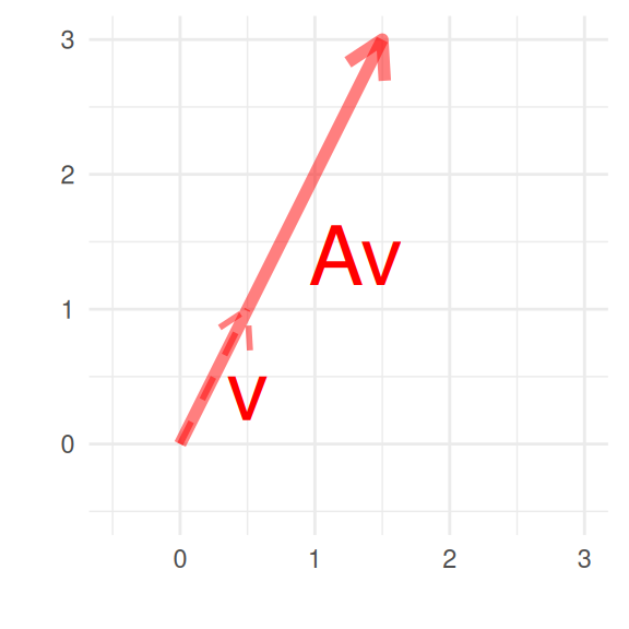
Eigen values, Eigen vectors

Consider a square matrix, \(A \in \R^{d\times d}\), and a nonzero vector, \(v \in \R^d\), \(v\) is an eigen vector for the eigen value \(\lambda\) if \[Av = \lambda v.\] If \(v\) is an eigen vector for \(A\), applying \(A\) to \(v\) just consists in multiplying by the corresponding eigen value.

  • Identify the eigen values and eigen vectors for \(A_1 = \begin{pmatrix}1 & 0 \cr 0 & 2\end{pmatrix}\), \(A_2 = \begin{pmatrix}1 & 3 \cr 0 & 2\end{pmatrix},\) \(A_3 = \begin{pmatrix} 2 & 2 \cr -2 & 2 \end{pmatrix}.\)

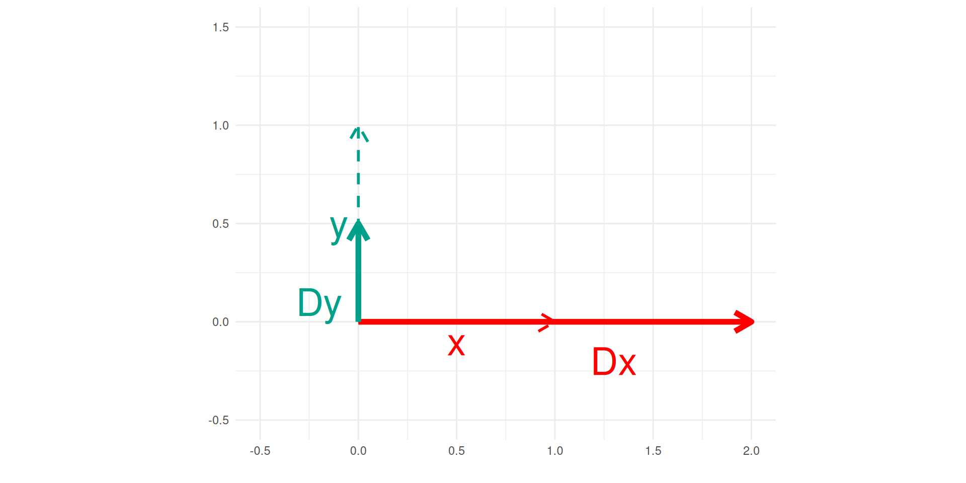
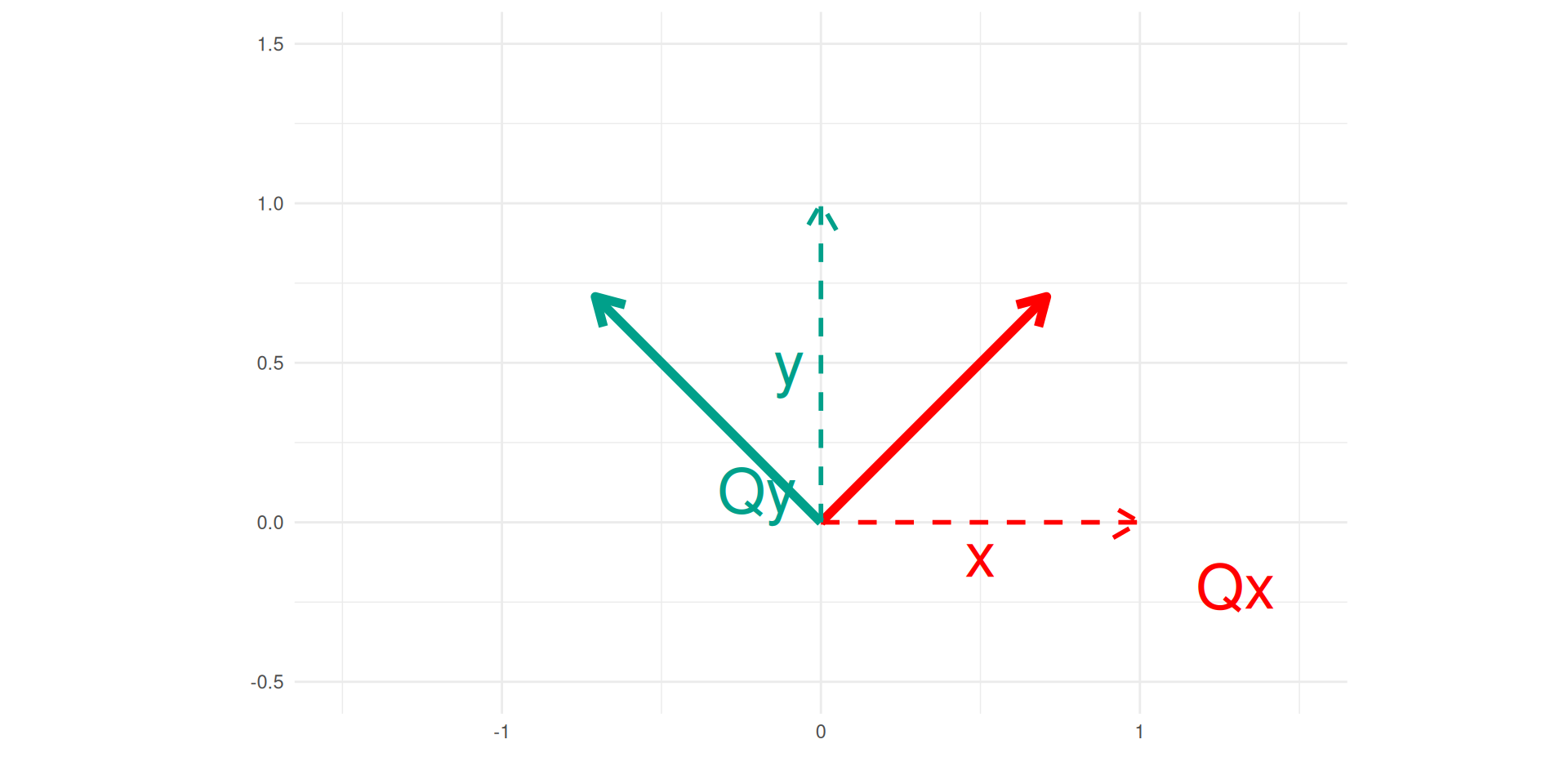
Singular Value Decomposition (SVD)

Let’s \(A\) a \(n\times d\) matrix of rank \(r\), there exists a \(n\times n\) orthogonal matrix \(P\), a \(d\times d\) orthogonal matrix \(Q\), and \(D_1\) a diagonal \(r\times r\) matrix whose diagonal terms are in decreasing order such that: \[ A = P \begin{pmatrix} D_1 & 0 \cr 0 & 0 \cr \end{pmatrix} Q^\intercal\]

For a nice and visual course on SVD see the Steve Brunton Youbube Channel on this subject!

\(A = \frac{\sqrt{2}}{6} \begin{pmatrix} 0 & 4 \cr 6 & 2 \cr -3 & -5 \end{pmatrix}\) then consider

\(P = \frac{1}{3} \begin{pmatrix} 1 & -2 & 2 \cr 2 & 2 & 1 \cr -2 & 1 & 2 \end{pmatrix}, \quad D = \begin{pmatrix} 2 & 0 \cr 0 & -1 \cr 0 & 0 \end{pmatrix}, \quad and \ Q = \frac{\sqrt{2}}{2} \begin{pmatrix} 1 & -1 \cr 1 & 1 \end{pmatrix}\)

if \(A\) is a \({d\times d}\) symmetric matrix

\[A = P D P^\intercal.\]

A =matrix(c(0, sqrt(2), - sqrt(2)/2, 2* sqrt(2)/3, sqrt(2)/3, -5*sqrt(2)/6), ncol = 2);A
           [,1]       [,2]
[1,]  0.0000000  0.9428090
[2,]  1.4142136  0.4714045
[3,] -0.7071068 -1.1785113
svd(A)
$d
[1] 2 1

$u
           [,1]       [,2]
[1,] -0.3333333  0.6666667
[2,] -0.6666667 -0.6666667
[3,]  0.6666667 -0.3333333

$v
           [,1]       [,2]
[1,] -0.7071068 -0.7071068
[2,] -0.7071068  0.7071068
array([[ 0.        ,  0.94280904],
       [ 1.41421356,  0.47140452],
       [-0.70710678, -1.1785113 ]])
[[-0.33333333  0.66666667  0.66666667]
 [-0.66666667 -0.66666667  0.33333333]
 [ 0.66666667 -0.33333333  0.66666667]]
[2. 1.]
[[-0.70710678 -0.70710678]
 [-0.70710678  0.70710678]]

And now

It’s time to use this concept for Data Analysis

Bibliography

Banerjee, S. and A. Roy (2014). Linear algebra and matrix analysis for statistics. Vol. 181. Crc Press Boca Raton.

Cohen, M. X. (2022). Practical linear algebra for data science. O’Reilly Media, Inc.

Gentle, J. E. (2007). “Matrix algebra”. In: Springer texts in statistics, Springer, New York, NY, doi 10, pp. 978-0.

Harville, D. A. (1998). Matrix algebra from a statistician’s perspective.

Petersen, K. B., M. S. Pedersen, and others (2008). “The matrix cookbook”. In: Technical University of Denmark 7.15, p. 510.

Yoshida, R. (2021). Linear algebra and its applications with R. Chapman and Hall/CRC. URL: https://shainarace.github.io/LinearAlgebra/.