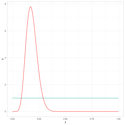
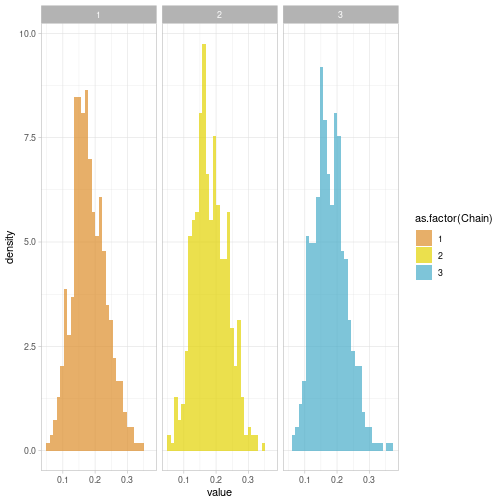
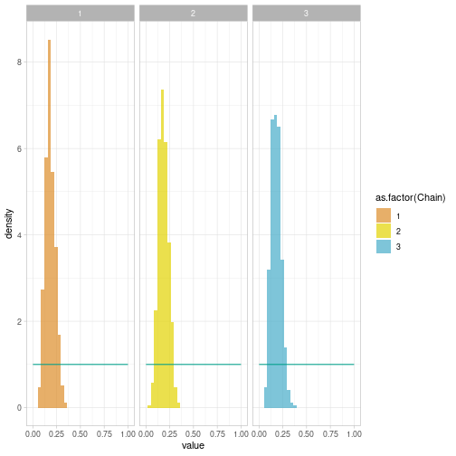
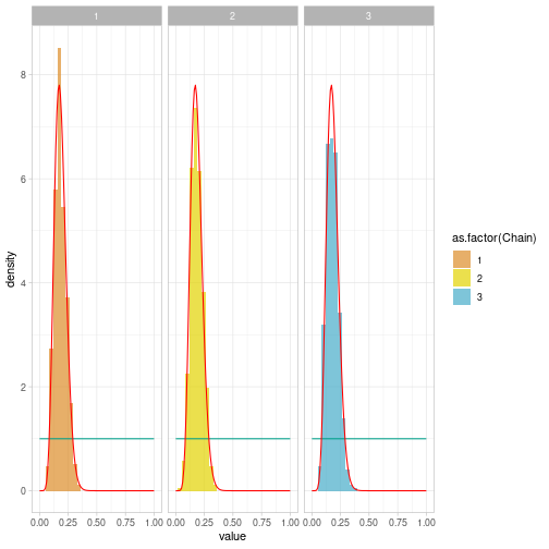
Building and estimating a first Bayesian model

class: center, middle, inverse, title-slide

# Building and estimating a first Bayesian model
### Marie-Pierre Etienne, Etienne Rivot
### <a href="https://marieetienne.github.io/bayesian_and_ecology" class="uri">https://marieetienne.github.io/bayesian_and_ecology</a>
### M2 Mode - Data science

---

---
name: coin 
# Tossing a coin
--

While tossing a coin 53 times, we got 9 tails. What could we say on the probability to get a tail ?
## Model of experiment

We model the experiment by 
$$ Y \sim \mathcal{B}(m, p),$$ 
with `$p$` the probability to get a tail and `$m$` the total number of trials.

---
template: coin
## Modelling the prior knowledge on `$p$`

As we never used that coin, we would like to add no information in the prior information. FIrst guess

$$ p \sim \mathcal{U}(0,1)$$

which is equivalent to

$$ p \sim \mathcal{B}eta(1,1)$$
---
template: coin
## Theoretical posterior distribution

The full bayesian specification for the model is a so called beta binomial model which has analytical posterior distribution.

`$$\pi(p\vert  Y_{obs}) \sim \mathcal{B}eta(Y_{obs} + 1,  m-Y_{obs} +1)$$`
---
template: coin
## Theoretical posterior distribution

Graphically

```r
Y <- 9
m <- 53
```

![](IllustrationMCMC_files/figure-html/unnamed-chunk-1-1.png)

---
name: sampling
# Sampling from the posterior distribution

--
## Practical Model specification

```r
model <- "
model{

## model 
  Y ~ dbinom(p, m)

## Prior distribution
  p ~ dbeta(1, 1)

} # end model
"
```

---
template: sampling
## Data specification

```r
data_list <- list(
  m = 53,
  Y = 9
)
```

---
template: sampling
## Initialisation

```r
init_list <- list(
  p=0.1
)
```

---
template: sampling
## Combining, model and data

```r
mjags <- jags.model(file=textConnection(model), 
                    data=data_list,
                    inits=init_list, 
                    n.chains = 3)
```

```
## Compiling model graph
##    Resolving undeclared variables
##    Allocating nodes
## Graph information:
##    Observed stochastic nodes: 1
##    Unobserved stochastic nodes: 1
##    Total graph size: 4
## 
## Initializing model
```

---
template: sampling
## Sampling from the posterior

We are interested in the posteriori distribution of `$p$`

```r
postSamples <- coda.samples(mjags, 
                            variable.names = c("p"),
                            n.iter = 50000, 
                            thin = 100)
```

---
template: sampling
## Comparing sampled and theoretical distributions

---

count: false

.panel1-post_sample-auto[

```r
## a nicer format
*postSamples_df <-  postSamples %>% ggs()
```
]
 
.panel2-post_sample-auto[

]

---
count: false

.panel1-post_sample-auto[

```r
## a nicer format
postSamples_df <-  postSamples %>% ggs()

*postSamples_df
```
]
 
.panel2-post_sample-auto[

```
## # A tibble: 1,500 x 4
##    Iteration Chain Parameter  value
##        <int> <int> <fct>      <dbl>
##  1         1     1 p         0.104 
##  2         2     1 p         0.187 
##  3         3     1 p         0.209 
##  4         4     1 p         0.0970
##  5         5     1 p         0.142 
##  6         6     1 p         0.163 
##  7         7     1 p         0.138 
##  8         8     1 p         0.146 
##  9         9     1 p         0.179 
## 10        10     1 p         0.169 
## # … with 1,490 more rows
```
]

---
count: false

.panel1-post_sample-auto[

```r
## a nicer format
postSamples_df <-  postSamples %>% ggs()

postSamples_df %>%
* ggplot()
```
]
 
.panel2-post_sample-auto[
![](IllustrationMCMC_files/figure-html/post_sample_auto_03_output-1.png)
]

---
count: false

.panel1-post_sample-auto[

```r
## a nicer format
postSamples_df <-  postSamples %>% ggs()

postSamples_df %>%
  ggplot() +
* facet_wrap(~as.factor(Chain))
```
]
 
.panel2-post_sample-auto[
![](IllustrationMCMC_files/figure-html/post_sample_auto_04_output-1.png)
]

---
count: false

.panel1-post_sample-auto[

```r
## a nicer format
postSamples_df <-  postSamples %>% ggs()

postSamples_df %>%
  ggplot() +
  facet_wrap(~as.factor(Chain)) +
* geom_histogram(data = postSamples_df, aes(x= value, y =..density.., fill = as.factor(Chain)), position = "identity", alpha = 0.7) + scale_fill_manual(values = wesanderson::wes_palette("FantasticFox1", n = 5))
```
]
 
.panel2-post_sample-auto[

```
## Scale for 'fill' is already present. Adding another scale for 'fill', which
## will replace the existing scale.
```

```
## `stat_bin()` using `bins = 30`. Pick better value with `binwidth`.
```

![](IllustrationMCMC_files/figure-html/post_sample_auto_05_output-1.png)
]

---
count: false

.panel1-post_sample-auto[

```r
## a nicer format
postSamples_df <-  postSamples %>% ggs()

postSamples_df %>%
  ggplot() +
  facet_wrap(~as.factor(Chain)) +
  geom_histogram(data = postSamples_df, aes(x= value, y =..density.., fill = as.factor(Chain)), position = "identity", alpha = 0.7) + scale_fill_manual(values = wesanderson::wes_palette("FantasticFox1", n = 5)) +
* stat_prior
```
]
 
.panel2-post_sample-auto[

```
## Scale for 'fill' is already present. Adding another scale for 'fill', which
## will replace the existing scale.
```

```
## `stat_bin()` using `bins = 30`. Pick better value with `binwidth`.
```

![](IllustrationMCMC_files/figure-html/post_sample_auto_06_output-1.png)
]

---
count: false

.panel1-post_sample-auto[

```r
## a nicer format
postSamples_df <-  postSamples %>% ggs()

```
## Scale for 'fill' is already present. Adding another scale for 'fill', which
## will replace the existing scale.
```

```
## `stat_bin()` using `bins = 30`. Pick better value with `binwidth`.
```

![](IllustrationMCMC_files/figure-html/post_sample_auto_07_output-1.png)
]

---
name: CMR
# Capture Mak Recapture

While monitoring a large population of size `$n$` unknown, `$m$` individuals have been marked and released.
The population might be considered as `$m$` marked individuals and `$n-m$` unmarked individuals. 
A recapture experiment leads to `$YM$` marked animals and `$YNM$` unmarked.

m = 53, YM = 9 and YNM = 75 ?

What is the size of the population ?
Under what assumptions ?

---
template: CMR
## Estimating the capture efficiency

The probability of capture might be infered from the recapture dataset and the experiment might be modelled as 
`\begin{equation}
 YM \sim \mathcal{B}(m, p).
\end{equation}`

The capture mark recapture experiment has been used for the first time on these conditions. Few is known on the probability of capture. Therefore an uniform prior is chosen to model the a priori knowledge on `$p$`.

---
template: CMR
## Data

```r
m <- 53
YM <- 9
```

---
template: CMR
## Let's figure out the rest of the model