library(Rhabit)
library(viridis)
library(ggplot2)
library(gridExtra)
library(abind)
library(dplyr)

This vignette illustrates the use of the Rhabit package to simulate data from a Langevin model and to estimate the parameters.

Simulation of the Langevin model

In the Langevin model, we assume that the movement is directed by a field of covariates. Those fields of covariates are mandatory to simulate a path according to the model.

Simulating covariate fields

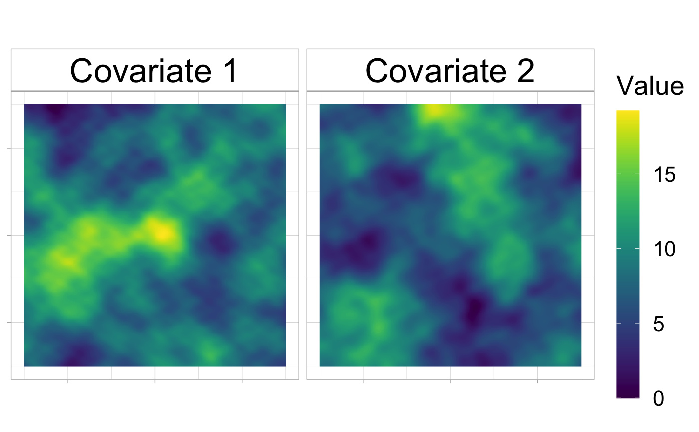
In the presented example, the path is observed on a square, centered on the origine and whose sides equal 30.

In order to g a enerate a field of covariates, we propose to simulate two Mattern processes with the same parameters parameters \((\rho, \nu, \sigma^2)\) The covriates are obtained by applying a log transformation to the square of the Mattern process.

set.seed(1)# repeatability
lim <- c(-15, 15, -15, 15) # limits of map
resol <- 0.1 # grid resolution
rho <- 4; nu <- 1.5; sigma2 <- 10# Matern covariance parameters
mean_function <- function(z){# mean function
  -log(3 + sum(z^2))
}
J <- 2 # number of covariates

Then, simulating

covariates <- replicate(J,
                        simSpatialCov(lim, nu, rho, sigma2, resol = resol,
                                      mean_function = mean_function,
                                      raster_like = T),
                        simplify = F)

The resulting covariates are available in the package~:

data("covariates", package = "Rhabit")

Representation of the fileds of covariates

ggopts <- theme_light()+theme(text = element_text(size = 20),
                axis.text = element_blank(),
                axis.title = element_blank(),
                legend.key.height= unit(3, "line"),
                strip.background = element_rect(fill="white",colour = "grey") ,
                strip.text = element_text(size = 25, color = "black"))
levels <- factor(paste("Covariate", 1:J), levels = paste("Covariate", 1:J))
cov_df <- do.call(rbind.data.frame,
                 lapply(1:J,
                        function(j){
                          Rhabit::rasterToDataFrame(covariates[[j]], levels[j])
                        }))
ggplot(cov_df, aes(x,y)) + geom_raster(aes(fill = val)) +
  coord_equal() + scale_fill_viridis(name = "Value") + facet_wrap(level~.) +
  ggopts

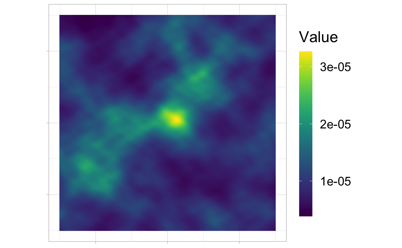
The resulting Utilization Distribution

\[\begin{equation} \rmd\X_t = \dfrac{\gamma^2}{2} \nabla \log \ud(\X_t) \rmd t + \gamma \rmd \bm{W}_t,\quad \X_0 =\bm{x}_0. \end{equation}\]

beta_true <- c(10, 5)
ud_rast <- covariates[[1]] # initialization
dx <- diff(ud_rast$x)[1]
dy <- diff(ud_rast$x)[1]
ud_rast$z <- exp(Reduce("+",
                    lapply(1:J, function(j)
                      dx * dy * beta_true[j] * covariates[[j]]$z)))
ud_rast$z <- ud_rast$z / sum(ud_rast$z)
ud_df <- rasterToDataFrame(ud_rast)
ggplot(ud_df, aes(x,y)) + geom_raster(aes(fill = val)) +
  coord_equal() + scale_fill_viridis(name = "Value") +
  ggopts

Simulation

Setting simulation parameters:

t_final <- 10
n_obs <- 10001
times <- seq(0, t_final, length.out = n_obs)

Then, one can simulate using cov_list

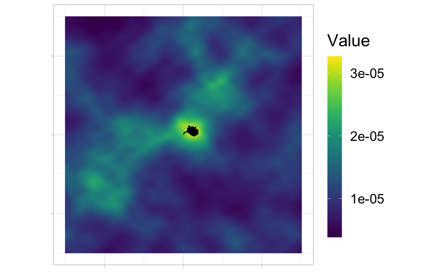
set.seed(1) #repeatability
tracks <- simLangevinMM(beta = beta_true, gamma2 = 10,
                        times = times, loc0 = c(0, 0),
                        cov_list = covariates, keep_grad = T)

These simulated tracks are a data set that can be loaded

data("tracks", package = "Rhabit")

And can be plotted

ggplot(ud_df, aes(x,y)) + geom_raster(aes(fill = val)) +
  coord_equal() + scale_fill_viridis(name = "Value") +
  geom_path(data = tracks[, 1:2]) +
  ggopts

Estimation

The dataset is expected to contain columns - x and y which specify the relocations - t , for the corresponding times - for each variable of interest, let’s say V1, two columns V1_x and V1_y which contain the computed gradient of covariates V1 at the recorded location.

## test with the formula
fitted_langevin <- fit_langevin_ud(
  cbind(x,y) ~ grad_c1 + grad_c2, data = tracks)

The effects of the covariates can be obtained via

coef(fitted_langevin)

  grad_c1   grad_c2 
10.426025  5.124737

while the speed parameter is obtained through

speed_coef(fitted_langevin)

[1] 10.03088

Testing thhe effects

The function tests for every covariate, if the corresponding parameter equals 0 or not.

The Null hypothesis for the speed parameter is \(\gamma^2 =0\).

summary(fitted_langevin)


Formula:
cbind(x, y) ~ grad_c1 + grad_c2

Coefficients:
         Estimate Std. Error  t value      Pr(>|t|)
grad_c1 10.426025  0.2546123 40.94864  0.000000e+00
grad_c2  5.124737  0.1414662 36.22588 2.243933e-278


Speed parameter:
       Estimate chi value Pr(>|t|)
gamma2 10.03088  200597.5        0

The confidence intervals for each parameter are available with.

fitted_langevin$CI

           0.025     0.975
grad_c1 9.926995 10.925056
grad_c2 4.847468  5.402005
gamma2  9.837136 10.230432

The expected trend in the movement at each observed location is given by

head(fitted_langevin$predicted, n = 10)

# A tibble: 10 x 4
      ID      x       y     t
   <dbl>  <dbl>   <dbl> <dbl>
 1     1 NA     NA      0    
 2     1  0.132  0.0869 0.001
 3     1  0.189  0.169  0.002
 4     1  0.205  0.375  0.003
 5     1  0.338  0.336  0.004
 6     1  0.478  0.435  0.005
 7     1  0.620  0.426  0.006
 8     1  0.842  0.480  0.007
 9     1  0.852  0.289  0.008
10     1  1.02   0.321  0.009

Simulation - Estimation of a full Langevin model

Pierre Gloaguen, Marie-Pierre Etienne