library(ggplot2)
library(ggfortify)
library(tidyverse)
library(car)
library(sf)

## Linking to GEOS 3.6.2, GDAL 2.2.3, PROJ 4.9.3

library(maps)

## 
## Attaching package: 'maps'

## The following object is masked from 'package:purrr':
## 
##     map

library(rnaturalearth)

Présentation

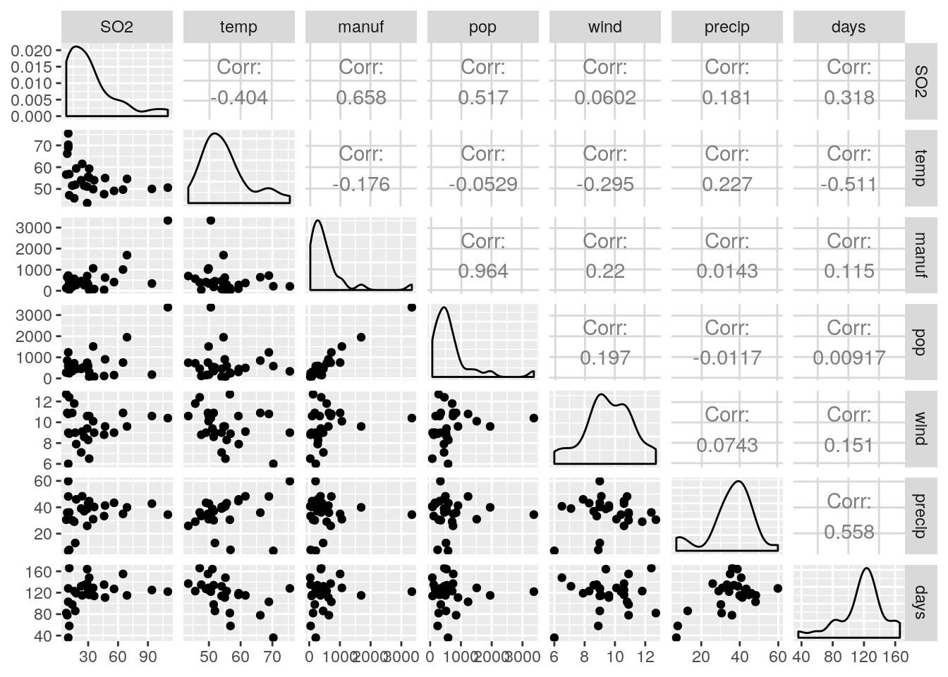
Pour étudier la pollution dans des villes américaine, on a mesuré différentes variables. Les valeurs présentées sont les moyennes annuelles des années 1969 à 1971.\ SO2 : Dyoxide de soufre augmente les risques de pluies acides\ temp : temperature \ manuf : nbre de societe employant plus de 20 salariés \ pop : population en milliers \ wind : vitesse moyenne du vent annuel en miles/Heure \ precip hauteur de precipitations annuelles en pouces \ days : nbre de jours de precipitations \

Chargement des données

usdata <- read.table("data/USAIR2.DAT",
                     skip = 8,
                     header = T,
                     sep = ";")

usdata <- usdata %>%  
  mutate(City = as.character(City)) 
head(usdata)

##            City SO2 temp manuf pop wind precip days
## 1       Phoenix  10 70.3   213 582  6.0   7.05   36
## 2   Little rock  13 61.0    91 132  8.2  48.52  100
## 3 San Francisco  12 56.7   453 716  8.7  20.66   67
## 4        Denver  17 51.9   454 515  9.0  12.95   86
## 5      Hartford  56 49.1   412 158  9.0  43.37  127
## 6    Wilmington  36 54.0    80  80  9.0  40.25  114

Representation des villes

##load us.cities 
data(us.cities)
nbCity <- dim(usdata)[1]
head(us.cities$name)

## [1] "Abilene TX" "Akron OH"   "Alameda CA" "Albany GA"  "Albany NY" 
## [6] "Albany OR"

##indices of studied cities in us.cities
ind.cities <- c(694, 509, 802, 247, 387, 990, 944, 429, 559, 41,
                173, 422, 248, 988, 522, 609, 55, 250, 568, 443,
                785, 650, 7, 5, 126, 180, 185, 195, 693, 700, 726,
                549, 601, 225, 413, 794, 619, 753, 834, 165, 567)

sites <- us.cities[ind.cities,] 


sites %>% 
  select(-pop) %>% 
  mutate(City = str_replace(name, pattern =  " [:upper:]+", ''))  -> sites

usdata <- inner_join(sites, usdata)

## Joining, by = "City"

world <- ne_countries(scale = "medium", returnclass = "sf")



ggplot(data = world) +
    geom_sf() +
    geom_point(data = usdata, aes(x = long, y = lat),
               size = 2, 
              shape = 21, fill = "darkred") +
    coord_sf(xlim = c(-130, -64), ylim = c(22, 50), expand = FALSE)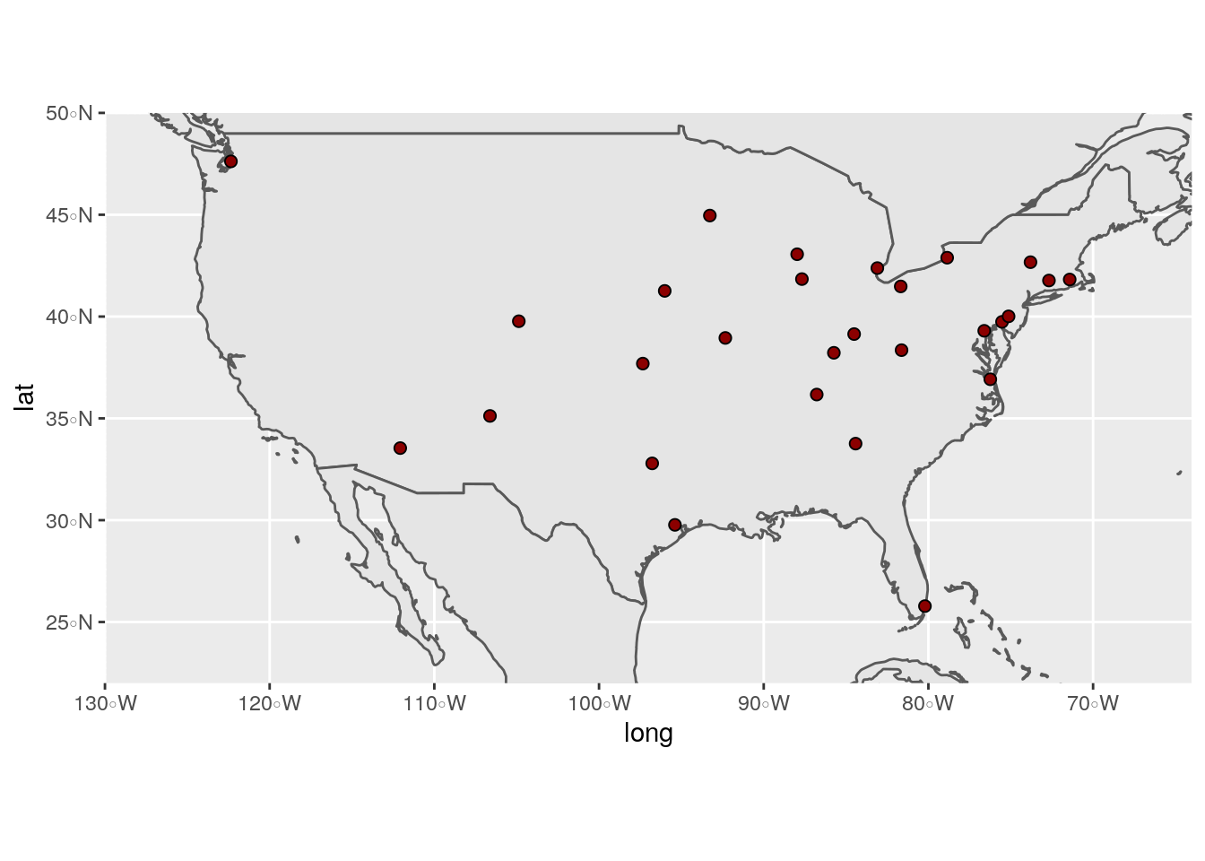

Description des données

Statistiques simples sur les données :

usdata %>%  summarise_if(is.numeric, mean, na.rm = TRUE)

##        lat      long   capital      SO2   temp    manuf      pop     wind
## 1 38.81321 -87.89321 0.5714286 32.67857 55.075 536.7857 670.1071 9.589286
##     precip     days
## 1 35.80929 117.1071

usdata %>%  summarise_if(is.numeric, sd, na.rm = TRUE)

##        lat     long   capital      SO2     temp    manuf      pop     wind
## 1 4.668694 12.62063 0.9200874 25.84864 7.649237 660.6569 680.2505 1.609541
##     precip     days
## 1 11.72057 29.27689

Etude de la corrélation entre les variables :

library(GGally)
usdata %>% select(-name, -country.etc, -capital, -City, -lat, -long) %>% ggpairs()

Visualisation de la pollution

world <- ne_countries(scale = "medium", returnclass = "sf")
ggplot(data = world) +
    geom_sf() +
    geom_point(data = usdata, aes(x = long, y = lat, size = log(SO2)),
              shape = 21) +
    coord_sf(xlim = c(-130, -64), ylim = c(22, 50), expand = FALSE)  +  theme(legend.position = 'bottom') + scale_fill_gradient(low="blue", high="red") + 
  labs( size="log(SO2)")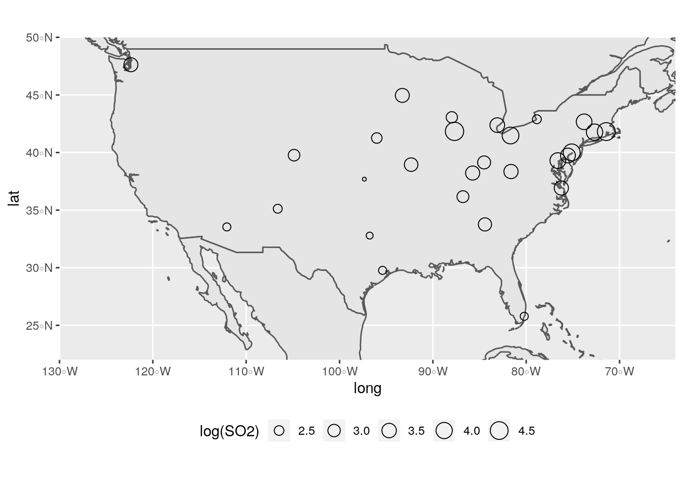

The size of the dots depends on the SO2 value and the color as well.

Visualisation du lien pollution et nombre d’usines

world <- ne_countries(scale = "medium", returnclass = "sf")
ggplot(data = world) +
    geom_sf() +
    geom_point(data = usdata, aes(x = long, y = lat, fill = manuf, size = log(SO2)),
              shape = 21) +
    coord_sf(xlim = c(-130, -64), ylim = c(22, 50), expand = FALSE)  +  theme(legend.position = "bottom") + scale_fill_viridis_c() +     
  labs( size="log(SO2)", fill = "Nombre d'usines")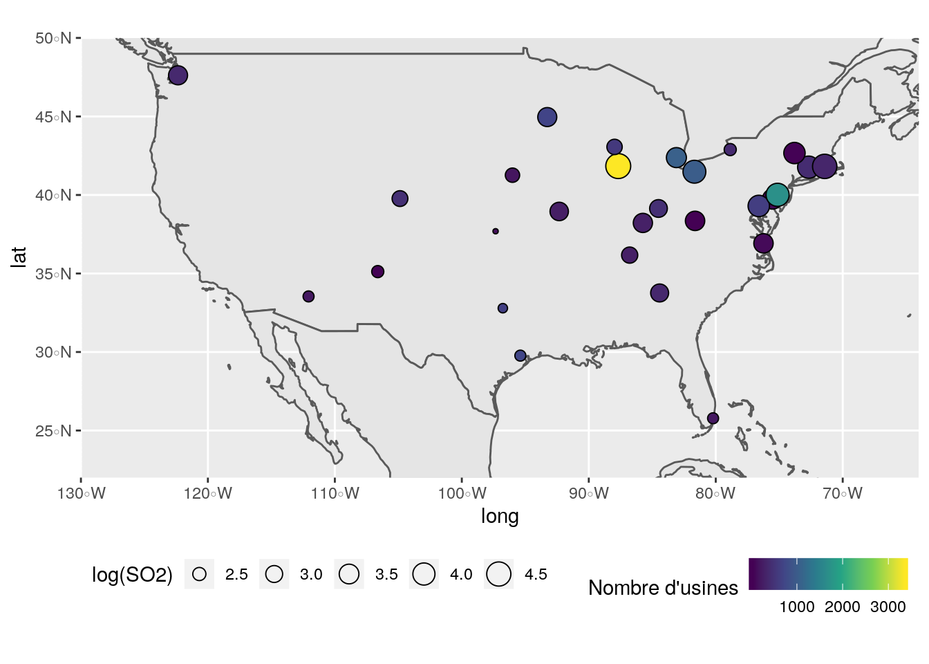

The size of the dots depends on the SO2 value and the color on the manuf variables value.

Régression linéaire simple

##regression SO2 en fonction de manuf

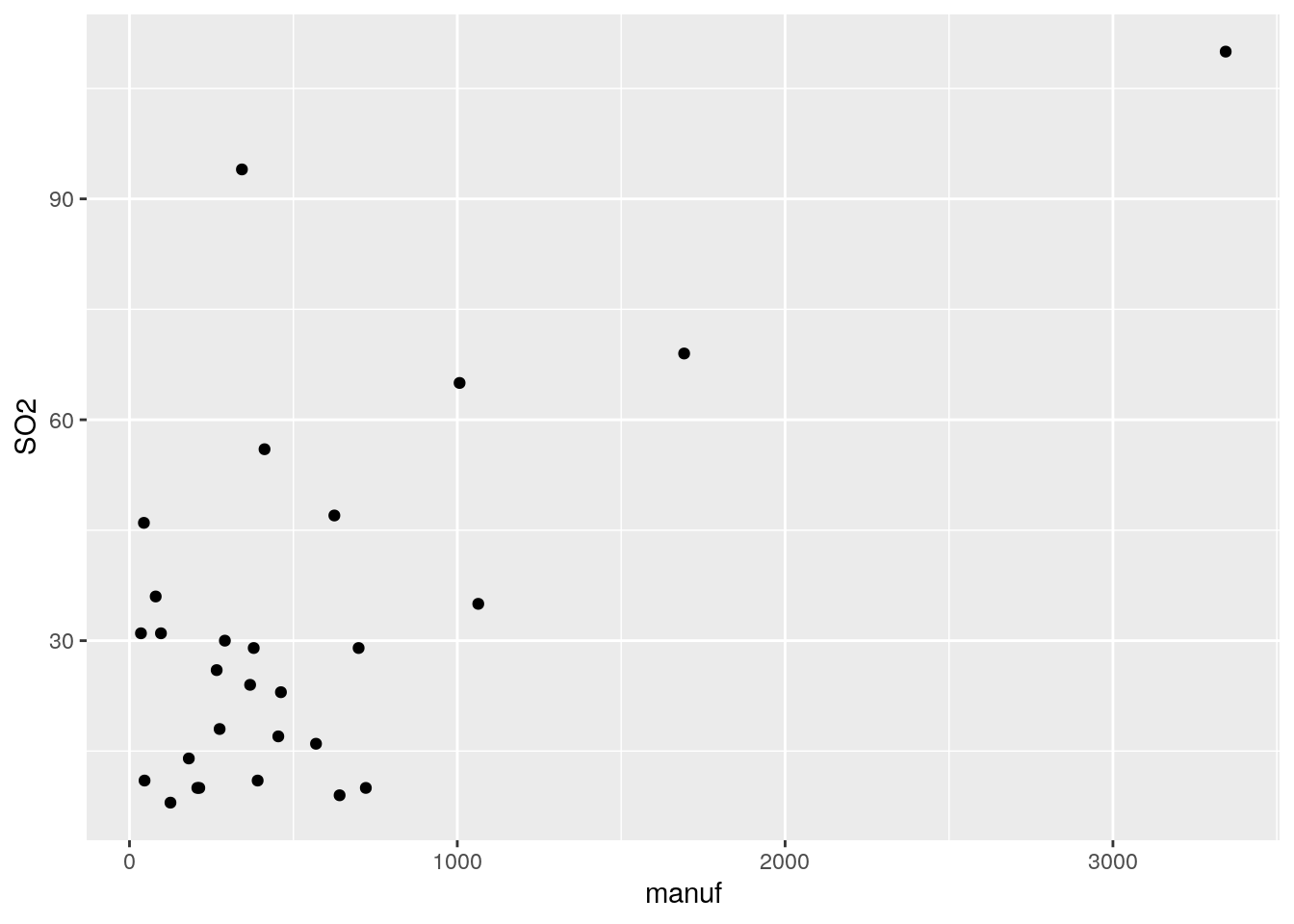
usdata %>% ggplot() + geom_point(aes(y=SO2, x =manuf))

Le SO2 en fonction du nombre d’entreprises.

us.lm <- lm(SO2 ~ manuf, data = usdata)
model.matrix(us.lm)

##    (Intercept) manuf
## 1            1   213
## 2            1   454
## 3            1   412
## 4            1    80
## 5            1   207
## 6            1   368
## 7            1  3344
## 8            1   125
## 9            1   291
## 10           1   625
## 11           1  1064
## 12           1   699
## 13           1   181
## 14           1    46
## 15           1    44
## 16           1   391
## 17           1   462
## 18           1  1007
## 19           1   266
## 20           1  1692
## 21           1   343
## 22           1   275
## 23           1   641
## 24           1   721
## 25           1    96
## 26           1   379
## 27           1    35
## 28           1   569
## attr(,"assign")
## [1] 0 1

summary(us.lm)

## 
## Call:
## lm(formula = SO2 ~ manuf, data = usdata)
## 
## Residuals:
##     Min      1Q  Median      3Q     Max 
## -27.422 -13.679  -6.043  10.064  66.311 
## 
## Coefficients:
##              Estimate Std. Error t value Pr(>|t|)    
## (Intercept) 18.857158   4.864747   3.876 0.000645 ***
## manuf        0.025748   0.005777   4.457 0.000141 ***
## ---
## Signif. codes:  0 '***' 0.001 '**' 0.01 '*' 0.05 '.' 0.1 ' ' 1
## 
## Residual standard error: 19.83 on 26 degrees of freedom
## Multiple R-squared:  0.4331, Adjusted R-squared:  0.4113 
## F-statistic: 19.86 on 1 and 26 DF,  p-value: 0.000141

Comparaison modèle nul et modèle incluant le nombre d’usines

lm0 <- lm(SO2 ~ 1, data = usdata)
anova(lm0, us.lm)

## Analysis of Variance Table
## 
## Model 1: SO2 ~ 1
## Model 2: SO2 ~ manuf
##   Res.Df   RSS Df Sum of Sq      F   Pr(>F)    
## 1     27 18040                                 
## 2     26 10227  1      7813 19.863 0.000141 ***
## ---
## Signif. codes:  0 '***' 0.001 '**' 0.01 '*' 0.05 '.' 0.1 ' ' 1

Valeur des paramètres estimés et tests sur les paramètres :

summary(us.lm)

## 
## Call:
## lm(formula = SO2 ~ manuf, data = usdata)
## 
## Residuals:
##     Min      1Q  Median      3Q     Max 
## -27.422 -13.679  -6.043  10.064  66.311 
## 
## Coefficients:
##              Estimate Std. Error t value Pr(>|t|)    
## (Intercept) 18.857158   4.864747   3.876 0.000645 ***
## manuf        0.025748   0.005777   4.457 0.000141 ***
## ---
## Signif. codes:  0 '***' 0.001 '**' 0.01 '*' 0.05 '.' 0.1 ' ' 1
## 
## Residual standard error: 19.83 on 26 degrees of freedom
## Multiple R-squared:  0.4331, Adjusted R-squared:  0.4113 
## F-statistic: 19.86 on 1 and 26 DF,  p-value: 0.000141

Effet levier des différents individus

autoplot(us.lm)

 h.us.lm <- hatvalues(us.lm)
 sum(h.us.lm)

## [1] 2

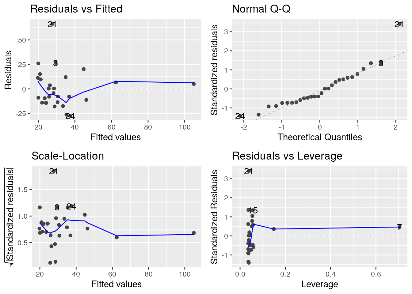
 sum(h.us.lm)/length(usdata$SO2)

## [1] 0.07142857

Graphiques de diagnostics

autoplot(us.lm, data = usdata)

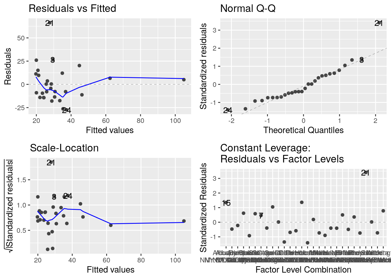
Les différents graphiques de diagnostic fournis par R

Effet de la ville de chicago

usdata %>% mutate(id = rownames(usdata)) %>% filter(id != 'Chicago') -> usdata_sans_chicago
lm_sans_chicago <- lm(SO2 ~ manuf , data = usdata_sans_chicago)
summary(lm_sans_chicago)

## 
## Call:
## lm(formula = SO2 ~ manuf, data = usdata_sans_chicago)
## 
## Residuals:
##     Min      1Q  Median      3Q     Max 
## -27.422 -13.679  -6.043  10.064  66.311 
## 
## Coefficients:
##              Estimate Std. Error t value Pr(>|t|)    
## (Intercept) 18.857158   4.864747   3.876 0.000645 ***
## manuf        0.025748   0.005777   4.457 0.000141 ***
## ---
## Signif. codes:  0 '***' 0.001 '**' 0.01 '*' 0.05 '.' 0.1 ' ' 1
## 
## Residual standard error: 19.83 on 26 degrees of freedom
## Multiple R-squared:  0.4331, Adjusted R-squared:  0.4113 
## F-statistic: 19.86 on 1 and 26 DF,  p-value: 0.000141

Régression multiple

Mise en oeuvre de la régression multiple :

us.lm2 <- lm(SO2 ~ temp + manuf + wind + precip + days, data = usdata)
## test de type I
anova(us.lm2)

## Analysis of Variance Table
## 
## Response: SO2
##           Df Sum Sq Mean Sq F value   Pr(>F)    
## temp       1 2939.4  2939.4 10.5638  0.00367 ** 
## manuf      1 6417.5  6417.5 23.0635 8.51e-05 ***
## wind       1  529.0   529.0  1.9010  0.18182    
## precip     1 1361.2  1361.2  4.8919  0.03767 *  
## days       1  671.4   671.4  2.4128  0.13461    
## Residuals 22 6121.6   278.3                     
## ---
## Signif. codes:  0 '***' 0.001 '**' 0.01 '*' 0.05 '.' 0.1 ' ' 1

## test de type II
Anova(us.lm2, type="II")

## Anova Table (Type II tests)
## 
## Response: SO2
##           Sum Sq Df F value    Pr(>F)    
## temp      2739.4  1  9.8449  0.004784 ** 
## manuf     6730.1  1 24.1867 6.427e-05 ***
## wind      1077.8  1  3.8734  0.061787 .  
## precip    1807.1  1  6.4944  0.018317 *  
## days       671.4  1  2.4128  0.134613    
## Residuals 6121.6 22                      
## ---
## Signif. codes:  0 '***' 0.001 '**' 0.01 '*' 0.05 '.' 0.1 ' ' 1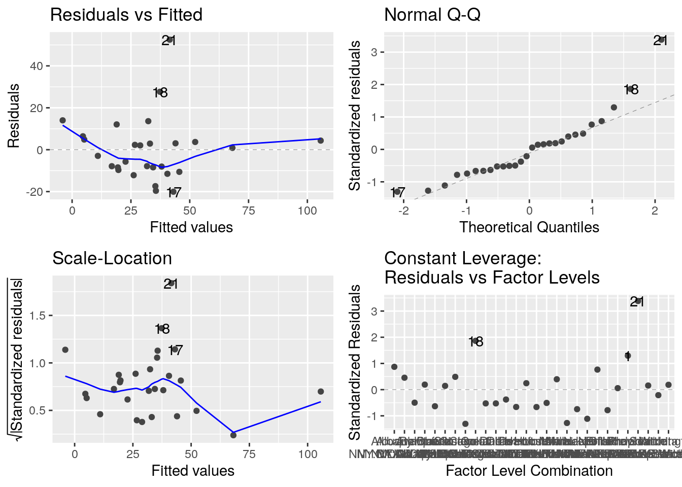

autoplot(us.lm2, data = usdata)

Les valeurs estimées des paramètres

summary(us.lm2)

## 
## Call:
## lm(formula = SO2 ~ temp + manuf + wind + precip + days, data = usdata)
## 
## Residuals:
##     Min      1Q  Median      3Q     Max 
## -20.058  -8.758  -1.047   4.467  52.507 
## 
## Coefficients:
##              Estimate Std. Error t value Pr(>|t|)    
## (Intercept) 185.97504   60.38787   3.080  0.00548 ** 
## temp         -2.35969    0.75206  -3.138  0.00478 ** 
## manuf         0.02469    0.00502   4.918 6.43e-05 ***
## wind         -4.31314    2.19153  -1.968  0.06179 .  
## precip        1.25036    0.49064   2.548  0.01832 *  
## days         -0.34159    0.21990  -1.553  0.13461    
## ---
## Signif. codes:  0 '***' 0.001 '**' 0.01 '*' 0.05 '.' 0.1 ' ' 1
## 
## Residual standard error: 16.68 on 22 degrees of freedom
## Multiple R-squared:  0.6607, Adjusted R-squared:  0.5835 
## F-statistic: 8.567 on 5 and 22 DF,  p-value: 0.0001267

Sélection automatique de variables

Sélection de variables backward : {

stepus.back <- step(us.lm2, direction = "backward")

## Start:  AIC=162.85
## SO2 ~ temp + manuf + wind + precip + days
## 
##          Df Sum of Sq     RSS    AIC
## <none>                 6121.6 162.85
## - days    1     671.4  6793.0 163.76
## - wind    1    1077.8  7199.4 165.39
## - precip  1    1807.1  7928.7 168.09
## - temp    1    2739.4  8861.0 171.20
## - manuf   1    6730.1 12851.7 181.61

Sélection de variables forward :

stepus.forward <- step(lm(SO2~1,data=usdata), scope=~temp+pop+manuf+wind+precip+days
, direction="forward")

## Start:  AIC=183.11
## SO2 ~ 1
## 
##          Df Sum of Sq   RSS    AIC
## + manuf   1    7813.0 10227 169.22
## + pop     1    4817.1 13223 176.41
## + temp    1    2939.4 15101 180.13
## + days    1    1827.9 16212 182.12
## <none>                18040 183.11
## + precip  1     594.1 17446 184.17
## + wind    1      65.3 17975 185.01
## 
## Step:  AIC=169.22
## SO2 ~ manuf
## 
##          Df Sum of Sq     RSS    AIC
## + pop     1    3597.9  6629.2 159.08
## + temp    1    1543.9  8683.2 166.63
## + days    1    1075.5  9151.5 168.10
## <none>                10227.1 169.22
## + precip  1     534.2  9692.8 169.71
## + wind    1     136.1 10091.0 170.84
## 
## Step:  AIC=159.08
## SO2 ~ manuf + pop
## 
##          Df Sum of Sq    RSS    AIC
## <none>                6629.2 159.08
## + precip  1    302.95 6326.3 159.77
## + wind    1    232.01 6397.2 160.08
## + temp    1    192.62 6436.6 160.25
## + days    1    106.51 6522.7 160.62

Sélection de variables stepwise :

stepus.stepwise <- step(us.lm2, direction="both")

## Start:  AIC=162.85
## SO2 ~ temp + manuf + wind + precip + days
## 
##          Df Sum of Sq     RSS    AIC
## <none>                 6121.6 162.85
## - days    1     671.4  6793.0 163.76
## - wind    1    1077.8  7199.4 165.39
## - precip  1    1807.1  7928.7 168.09
## - temp    1    2739.4  8861.0 171.20
## - manuf   1    6730.1 12851.7 181.61

Test sur le modèle sélectionné par la procédure

lm_select <- lm(SO2 ~ temp + manuf + pop + wind + precip, data = usdata)
summary(lm_select)

## 
## Call:
## lm(formula = SO2 ~ temp + manuf + pop + wind + precip, data = usdata)
## 
## Residuals:
##     Min      1Q  Median      3Q     Max 
## -24.568  -9.877  -0.007   4.942  47.822 
## 
## Coefficients:
##             Estimate Std. Error t value Pr(>|t|)   
## (Intercept) 84.56908   35.16231   2.405  0.02502 * 
## temp        -0.84103    0.49267  -1.707  0.10188   
## manuf        0.07234    0.02013   3.594  0.00161 **
## pop         -0.04709    0.01931  -2.439  0.02327 * 
## wind        -3.07932    2.01586  -1.528  0.14088   
## precip       0.46595    0.27440   1.698  0.10359   
## ---
## Signif. codes:  0 '***' 0.001 '**' 0.01 '*' 0.05 '.' 0.1 ' ' 1
## 
## Residual standard error: 15.59 on 22 degrees of freedom
## Multiple R-squared:  0.7036, Adjusted R-squared:  0.6362 
## F-statistic: 10.44 on 5 and 22 DF,  p-value: 3.111e-05

lm_select <- lm(SO2 ~ temp + manuf + pop + precip, data = usdata)
summary(lm_select)

## 
## Call:
## lm(formula = SO2 ~ temp + manuf + pop + precip, data = usdata)
## 
## Residuals:
##     Min      1Q  Median      3Q     Max 
## -26.241 -10.353  -0.657   6.450  45.185 
## 
## Coefficients:
##             Estimate Std. Error t value Pr(>|t|)   
## (Intercept) 45.87841   25.08654   1.829  0.08043 . 
## temp        -0.61030    0.48234  -1.265  0.21844   
## manuf        0.07433    0.02066   3.598  0.00152 **
## pop         -0.05028    0.01975  -2.546  0.01806 * 
## precip       0.39658    0.27835   1.425  0.16765   
## ---
## Signif. codes:  0 '***' 0.001 '**' 0.01 '*' 0.05 '.' 0.1 ' ' 1
## 
## Residual standard error: 16.04 on 23 degrees of freedom
## Multiple R-squared:  0.6721, Adjusted R-squared:  0.6151 
## F-statistic: 11.79 on 4 and 23 DF,  p-value: 2.352e-05

lm_select <- lm(SO2 ~ temp + manuf + pop , data = usdata)
summary(lm_select)

## 
## Call:
## lm(formula = SO2 ~ temp + manuf + pop, data = usdata)
## 
## Residuals:
##     Min      1Q  Median      3Q     Max 
## -24.746 -10.357  -0.267   6.538  47.182 
## 
## Coefficients:
##             Estimate Std. Error t value Pr(>|t|)    
## (Intercept) 48.92559   25.52591   1.917  0.06726 .  
## temp        -0.39680    0.46821  -0.847  0.40510    
## manuf        0.08133    0.02049   3.969  0.00057 ***
## pop         -0.05678    0.01962  -2.894  0.00797 ** 
## ---
## Signif. codes:  0 '***' 0.001 '**' 0.01 '*' 0.05 '.' 0.1 ' ' 1
## 
## Residual standard error: 16.38 on 24 degrees of freedom
## Multiple R-squared:  0.6432, Adjusted R-squared:  0.5986 
## F-statistic: 14.42 on 3 and 24 DF,  p-value: 1.404e-05

lm_select <- lm(SO2 ~ manuf + pop , data = usdata)
summary(lm_select)

## 
## Call:
## lm(formula = SO2 ~ manuf + pop, data = usdata)
## 
## Residuals:
##     Min      1Q  Median      3Q     Max 
## -21.929 -13.158  -1.843   9.222  47.126 
## 
## Coefficients:
##             Estimate Std. Error t value Pr(>|t|)    
## (Intercept) 27.65985    4.65455   5.943 3.34e-06 ***
## manuf        0.08954    0.01796   4.987 3.86e-05 ***
## pop         -0.06424    0.01744  -3.684  0.00111 ** 
## ---
## Signif. codes:  0 '***' 0.001 '**' 0.01 '*' 0.05 '.' 0.1 ' ' 1
## 
## Residual standard error: 16.28 on 25 degrees of freedom
## Multiple R-squared:  0.6325, Adjusted R-squared:  0.6031 
## F-statistic: 21.52 on 2 and 25 DF,  p-value: 3.675e-06

Régression multiple

Marie-Pierre Etienne

Présentation

Representation des villes

Description des données

Statistiques simples sur les données :

Etude de la corrélation entre les variables :

Visualisation de la pollution

Visualisation du lien pollution et nombre d’usines

Régression linéaire simple

Effet levier des différents individus

Régression multiple

Sélection automatique de variables