Modèle linéaire Généralisé
Les grenouilles à pattes rouges de Californie
Présentation du problème
Les auteurs ont collecté dans la littérature et dans les archives des muséums, des informations sur la présence ou l’absence de grenouilles sauvages dans 237 points d’eau de Californie. Pour chacun des sites, on dispose donc de sa position (longitude + latitude) de la source de l’information (Museum, Literature, PersCom ou Field Note) ainsi que de l’information sur la présence/absence de grenouilles.\ On cherche à caractériser l’aire de répartition de cette espèce en étudiant comment varie la probabilité de trouver des grenouilles dans un point d’eau en fonction de la latitude et de la longitude. On pourra aussi se demander si les différentes sources d’information documentent les mêmes " types " de points d’eau. \ Les données se trouvent dans le fichier Grenouille.don \ Les colonnes sont : Source Source2 presabs(Présence/Absence) latitude longitude \
Analyse descriptive
Les données sont disponibles sur grenouille
Grenouille <- read.table(file.path('data', 'Grenouille.don'), sep="",header=TRUE)
n <- nrow(Grenouille)

summary(Grenouille)
## Source Source2 Status Latitude Longitude
## FieldNote : 10 MVZ :59 A:113 Min. :32.64 Min. :-123.0
## Literature: 7 Perscom:31 P:123 1st Qu.:34.39 1st Qu.:-121.8
## Museum :188 LACM :26 Median :35.47 Median :-120.4
## Perscom : 31 CAS-SU :15 Mean :35.92 Mean :-120.1
## SDNHM :15 3rd Qu.:37.72 3rd Qu.:-118.7
## UMMZ :12 Max. :40.49 Max. :-116.4
## (Other):78Grenouille %>% mutate(pres_bin = ifelse(Status=='A', 0, 1)) -> Grenouille
p <- ggplot(data=Grenouille, aes(x=Latitude, y=pres_bin)) + geom_point()
p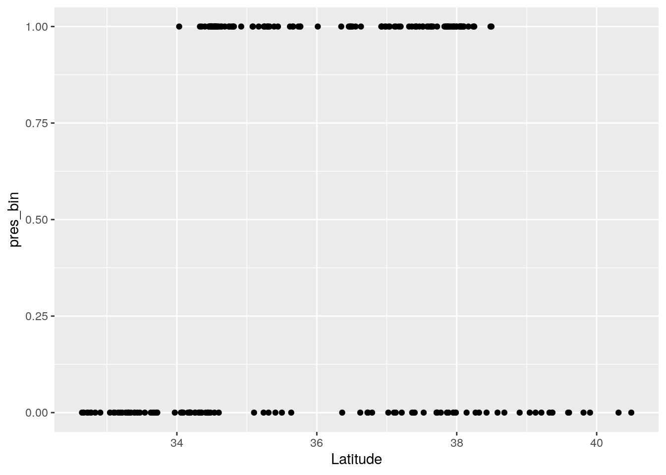
p <- ggplot(data=Grenouille, aes(y = Latitude, x = Longitude, col = Status)) + geom_point() + coord_fixed()
p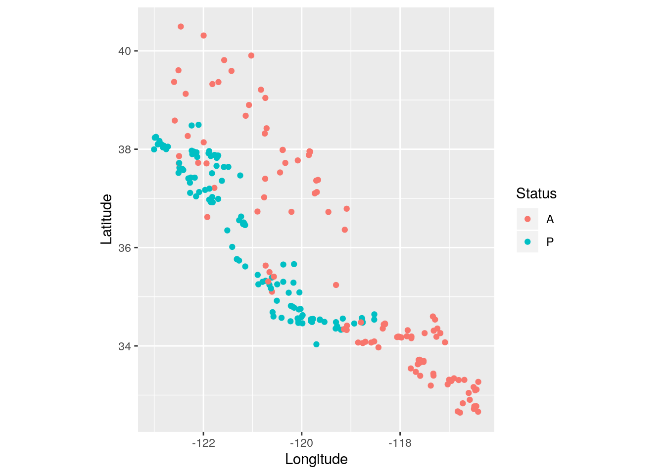
Etude de l’effet Latitude seule
\[ Y_k \overset{i.i.d}{\sim}\mathcal{B}(p_k), \quad logit(p_k) = \beta_0 + \beta_1 x^{(1)}_k \]
glm1  <-  glm(Status ~ Latitude, family = binomial, data=Grenouille)

glm0 <- glm(Status ~ 1, family = binomial, data=Grenouille)

summary(glm1)
##
## Call:
## glm(formula = Status ~ Latitude, family = binomial, data = Grenouille)
##
## Deviance Residuals:
## Min 1Q Median 3Q Max
## -1.635 -1.078 0.951 1.096 1.308
##
## Coefficients:
## Estimate Std. Error z value Pr(>|z|)
## (Intercept) -7.32756 2.52734 -2.899 0.00374 **
## Latitude 0.20645 0.07034 2.935 0.00334 **
## ---
## Signif. codes: 0 '***' 0.001 '**' 0.01 '*' 0.05 '.' 0.1 ' ' 1
##
## (Dispersion parameter for binomial family taken to be 1)
##
## Null deviance: 326.74 on 235 degrees of freedom
## Residual deviance: 317.81 on 234 degrees of freedom
## AIC: 321.81
##
## Number of Fisher Scoring iterations: 4## Analysis of Deviance Table
##
## Model 1: Status ~ 1
## Model 2: Status ~ Latitude
## Resid. Df Resid. Dev Df Deviance Pr(>Chi)
## 1 235 326.74
## 2 234 317.81 1 8.9292 0.002806 **
## ---
## Signif. codes: 0 '***' 0.001 '**' 0.01 '*' 0.05 '.' 0.1 ' ' 1new_data <- data.frame(Latitude = seq(0, 70, by = 0.1))
new_data %>% mutate(prediction = predict(glm1, newdata = new_data, type = 'response' ) ) -> new_data
ggplot(new_data) + geom_line(aes(x=Latitude, y = prediction)) + geom_point(data=Grenouille, aes(x=Latitude, y = pres_bin)) + xlim(c(33, 40))## Warning: Removed 630 rows containing missing values (geom_path).## Warning: Removed 11 rows containing missing values (geom_point).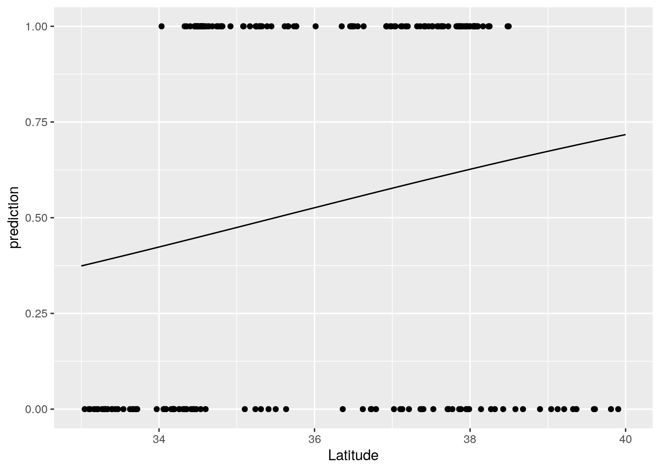
Introduction de la longitude
\[ Y_{k} \sim \mathcal{B}(p_k), \quad logit(p_k) = \beta_0 + \beta_1 x^{(1)}_k + \beta_2 x^{(2)}_k. \]
glm12  <-  glm(Status~Latitude+Longitude, family=binomial, data = Grenouille)

anova(glm1, glm12, test = 'Chisq')
## Analysis of Deviance Table
##
## Model 1: Status ~ Latitude
## Model 2: Status ~ Latitude + Longitude
## Resid. Df Resid. Dev Df Deviance Pr(>Chi)
## 1 234 317.81
## 2 233 146.81 1 171 < 2.2e-16 ***
## ---
## Signif. codes: 0 '***' 0.001 '**' 0.01 '*' 0.05 '.' 0.1 ' ' 1## Analysis of Deviance Table
##
## Model 1: Status ~ 1
## Model 2: Status ~ Longitude
## Resid. Df Resid. Dev Df Deviance
## 1 235 326.74
## 2 234 246.85 1 79.892## Analysis of Deviance Table
##
## Model 1: Status ~ 1
## Model 2: Status ~ Latitude
## Resid. Df Resid. Dev Df Deviance
## 1 235 326.74
## 2 234 317.81 1 8.9292## Analysis of Deviance Table
##
## Model 1: Status ~ Longitude
## Model 2: Status ~ Latitude + Longitude
## Resid. Df Resid. Dev Df Deviance Pr(>Chi)
## 1 234 246.85
## 2 233 146.81 1 100.04 < 2.2e-16 ***
## ---
## Signif. codes: 0 '***' 0.001 '**' 0.01 '*' 0.05 '.' 0.1 ' ' 1##
## Call:
## glm(formula = Status ~ Latitude + Longitude, family = binomial,
## data = Grenouille)
##
## Deviance Residuals:
## Min 1Q Median 3Q Max
## -2.6435 -0.3011 0.2393 0.4404 2.0575
##
## Coefficients:
## Estimate Std. Error z value Pr(>|z|)
## (Intercept) -265.0912 32.1226 -8.252 < 2e-16 ***
## Latitude -2.1157 0.3171 -6.671 2.53e-11 ***
## Longitude -2.8382 0.3523 -8.056 7.87e-16 ***
## ---
## Signif. codes: 0 '***' 0.001 '**' 0.01 '*' 0.05 '.' 0.1 ' ' 1
##
## (Dispersion parameter for binomial family taken to be 1)
##
## Null deviance: 326.74 on 235 degrees of freedom
## Residual deviance: 146.81 on 233 degrees of freedom
## AIC: 152.81
##
## Number of Fisher Scoring iterations: 6## Analysis of Deviance Table
##
## Model: binomial, link: logit
##
## Response: Status
##
## Terms added sequentially (first to last)
##
##
## Df Deviance Resid. Df Resid. Dev
## NULL 235 326.74
## Latitude 1 8.929 234 317.81
## Longitude 1 171.002 233 146.81## Analysis of Deviance Table (Type II tests)
##
## Response: Status
## LR Chisq Df Pr(>Chisq)
## Latitude 100.04 1 < 2.2e-16 ***
## Longitude 171.00 1 < 2.2e-16 ***
## ---
## Signif. codes: 0 '***' 0.001 '**' 0.01 '*' 0.05 '.' 0.1 ' ' 1Grenouille %>% mutate(pred = predict(glm12, Grenouille, type = 'response' )) -> Grenouille
ggplot(data = Grenouille) + geom_point(aes(x= Latitude, y = pres_bin) ) + geom_point(aes(x=Latitude, y = pred), col= 'red')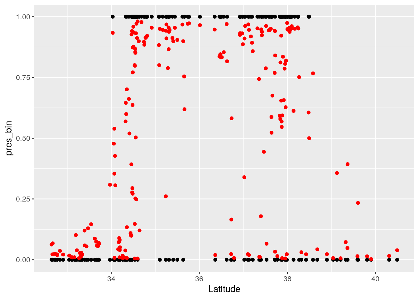
Etude des espèces de fourmis dans la forêt du Nourragues
Les données sont disponibles sur fourmis
Présentation du protocole
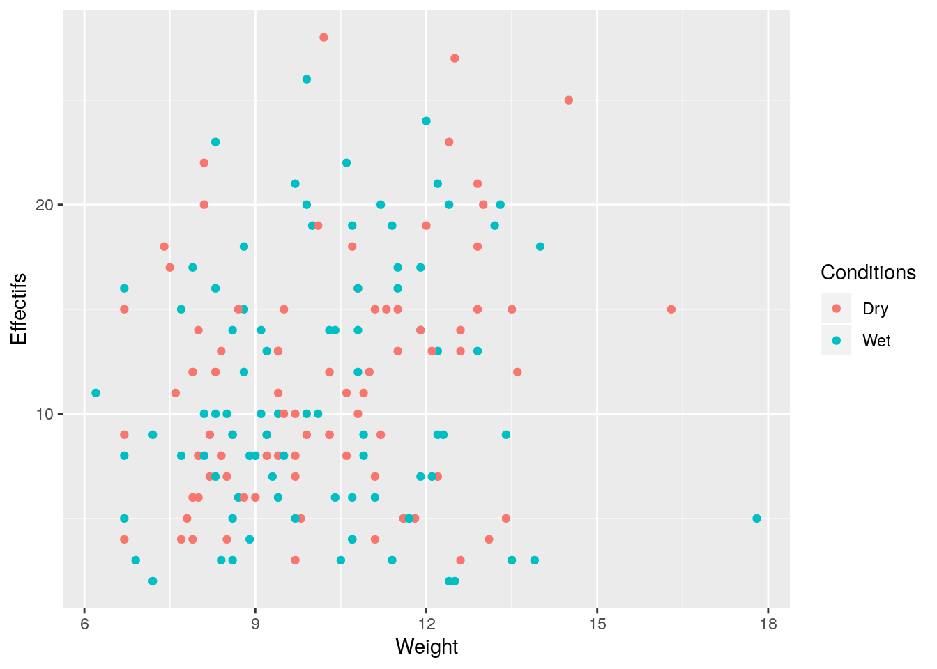
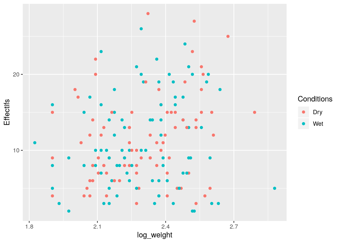
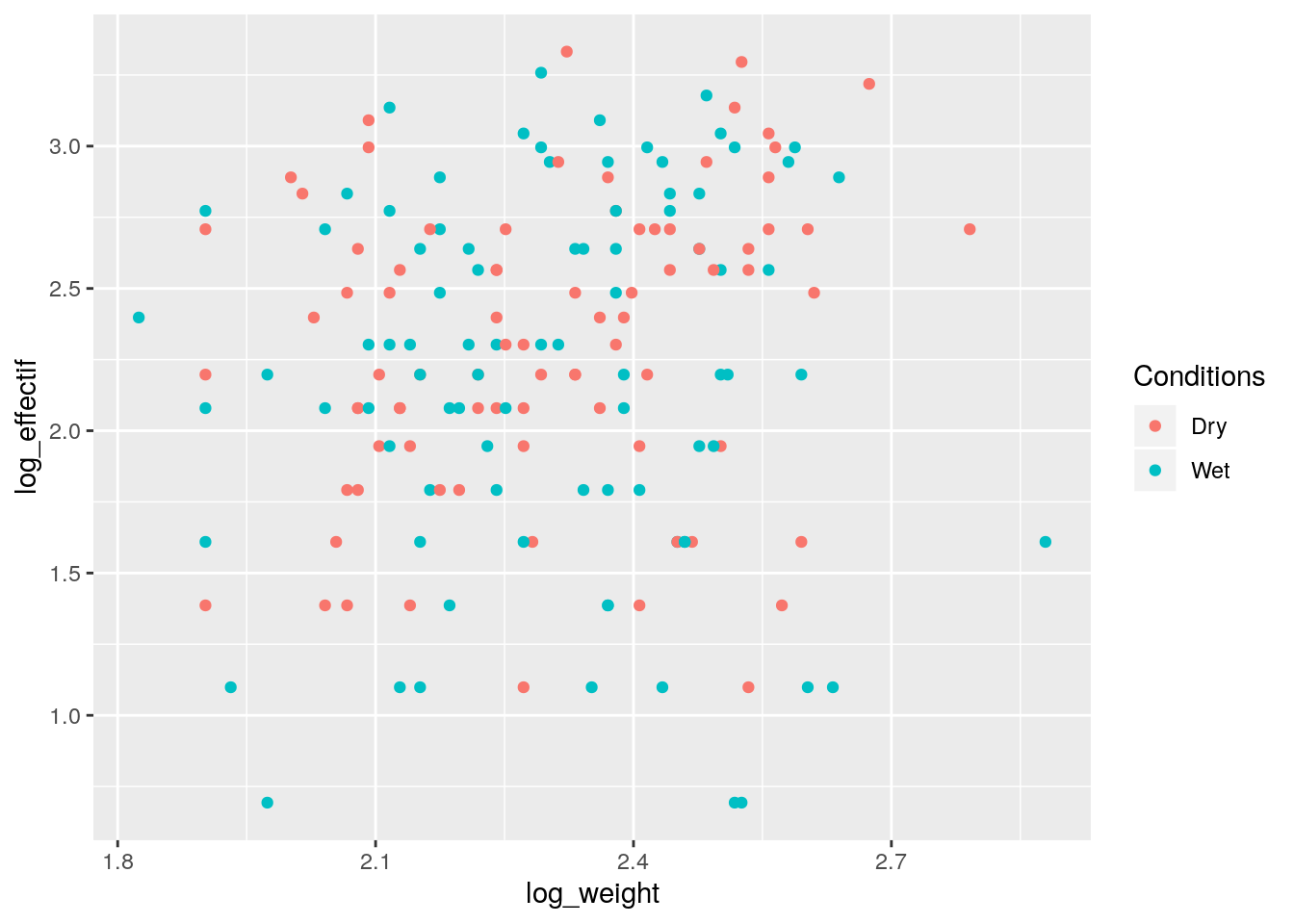
Le but de l’étude présentée est d’étudier la diversité des fourmis sur le site expérimental des Nourragues en Guyane Française. Le protocole expérimental suivant a été mis en place : on récolte \(1m^2\) de litière que l’on pèse. Le poids de litière (variable ) est vu comme un proxy (un indicateur) de l’épaisseur de la litière. On compte ensuite le nombre d’espèces différentes présentes dans l’échantillon (variable ). 50 points d’échantillonage distants d’au moins 10m ont été choisis :D’autre part, étant donnée la relative petite taille de la forêt d’Inselberg () seuls 20 points d’échantillonnage ont été sélectionnés pour ce site.
Enfin les conditions de recueil (humides ou sèches, variable ) ont été notées pour tester leur influence sur la présence des fourmis.
Analyse descriptive
Fourmis <- read.table(file.path('data','Fourmis.txt'),header=T, sep=',')


Fourmis %>% group_by(Site, Conditions) %>% summarise(n())
## # A tibble: 8 x 3
## # Groups: Site [4]
## Site Conditions `n()`
## <fct> <fct> <int>
## 1 FLWT Dry 24
## 2 FLWT Wet 26
## 3 FTWT Dry 24
## 4 FTWT Wet 26
## 5 GPWT Dry 22
## 6 GPWT Wet 28
## 7 INWT Dry 13
## 8 INWT Wet 7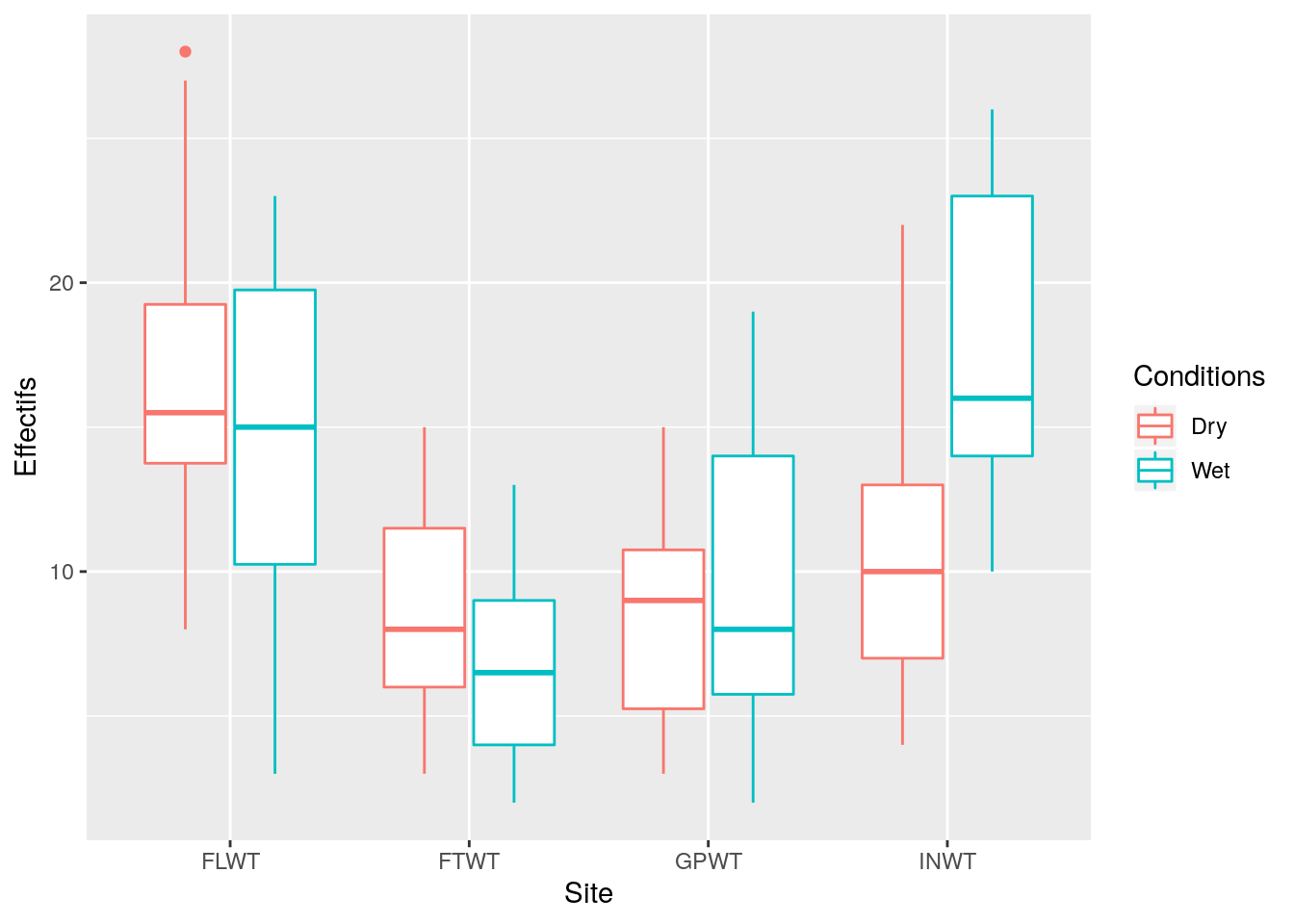
Que peut-on dire du plan d’expérience ?
Modélisation
Effet des conditions de recueil et du site
On modélise des comptages par des lois de Poisson
\[Y_{ijk} \overset{i.i.d}{\sim} \mathcal{P}(\lambda_{ij} E_{ijk})\]
glmInt <-  glm(Effectifs~Site*Conditions,offset=log(Weight),
             family="poisson", data=Fourmis )
summary(glmInt)
##
## Call:
## glm(formula = Effectifs ~ Site * Conditions, family = "poisson",
## data = Fourmis, offset = log(Weight))
##
## Deviance Residuals:
## Min 1Q Median 3Q Max
## -3.2267 -0.9268 -0.1522 0.8252 3.6257
##
## Coefficients:
## Estimate Std. Error z value Pr(>|z|)
## (Intercept) 0.49531 0.04969 9.968 < 2e-16 ***
## SiteFTWT -0.55200 0.08425 -6.552 5.69e-11 ***
## SiteGPWT -0.74225 0.08857 -8.380 < 2e-16 ***
## SiteINWT -0.38293 0.09727 -3.937 8.26e-05 ***
## ConditionsWet -0.02802 0.07132 -0.393 0.69438
## SiteFTWT:ConditionsWet -0.37426 0.12476 -3.000 0.00270 **
## SiteGPWT:ConditionsWet 0.16746 0.11880 1.410 0.15866
## SiteINWT:ConditionsWet 0.47387 0.14148 3.349 0.00081 ***
## ---
## Signif. codes: 0 '***' 0.001 '**' 0.01 '*' 0.05 '.' 0.1 ' ' 1
##
## (Dispersion parameter for poisson family taken to be 1)
##
## Null deviance: 534.13 on 169 degrees of freedom
## Residual deviance: 301.41 on 162 degrees of freedom
## AIC: 1017.2
##
## Number of Fisher Scoring iterations: 4## Analysis of Deviance Table
##
## Model: poisson, link: log
##
## Response: Effectifs
##
## Terms added sequentially (first to last)
##
##
## Df Deviance Resid. Df Resid. Dev
## NULL 169 534.13
## Site 3 201.731 166 332.40
## Conditions 1 0.000 165 332.40
## Site:Conditions 3 30.994 162 301.41## Analysis of Deviance Table (Type II tests)
##
## Response: Effectifs
## LR Chisq Df Pr(>Chisq)
## Site 200.543 3 < 2.2e-16 ***
## Conditions 0.000 1 0.9883
## Site:Conditions 30.994 3 8.526e-07 ***
## ---
## Signif. codes: 0 '***' 0.001 '**' 0.01 '*' 0.05 '.' 0.1 ' ' 1Effectif attendu
## $emmeans
##  Site Conditions  emmean     SE  df asymp.LCL asymp.UCL
##  FLWT Dry         0.4953 0.0497 Inf    0.3979    0.5927
##  FTWT Dry        -0.0567 0.0680 Inf   -0.1901    0.0767
##  GPWT Dry        -0.2469 0.0733 Inf   -0.3907   -0.1032
##  INWT Dry         0.1124 0.0836 Inf   -0.0515    0.2763
##  FLWT Wet         0.4673 0.0512 Inf    0.3670    0.5676
##  FTWT Wet        -0.4590 0.0765 Inf   -0.6089   -0.3091
##  GPWT Wet        -0.1075 0.0604 Inf   -0.2259    0.0109
##  INWT Wet         0.5582 0.0891 Inf    0.3836    0.7328
##
## Results are given on the log (not the response) scale.
## Confidence level used: 0.95
##
## $contrasts
##  contrast            estimate     SE  df z.ratio p.value
##  FLWT,Dry - FTWT,Dry   0.5520 0.0843 Inf  6.552  <.0001
##  FLWT,Dry - GPWT,Dry   0.7423 0.0886 Inf  8.380  <.0001
##  FLWT,Dry - INWT,Dry   0.3829 0.0973 Inf  3.937  0.0023
##  FLWT,Dry - FLWT,Wet   0.0280 0.0713 Inf  0.393  1.0000
##  FLWT,Dry - FTWT,Wet   0.9543 0.0912 Inf 10.464  <.0001
##  FLWT,Dry - GPWT,Wet   0.6028 0.0782 Inf  7.707  <.0001
##  FLWT,Dry - INWT,Wet  -0.0629 0.1020 Inf -0.617  1.0000
##  FTWT,Dry - GPWT,Dry   0.1902 0.1000 Inf  1.902  1.0000
##  FTWT,Dry - INWT,Dry  -0.1691 0.1078 Inf -1.568  1.0000
##  FTWT,Dry - FLWT,Wet  -0.5240 0.0851 Inf -6.155  <.0001
##  FTWT,Dry - FTWT,Wet   0.4023 0.1024 Inf  3.930  0.0024
##  FTWT,Dry - GPWT,Wet   0.0508 0.0910 Inf  0.558  1.0000
##  FTWT,Dry - INWT,Wet  -0.6149 0.1121 Inf -5.486  <.0001
##  GPWT,Dry - INWT,Dry  -0.3593 0.1112 Inf -3.231  0.0346
##  GPWT,Dry - FLWT,Wet  -0.7142 0.0894 Inf -7.988  <.0001
##  GPWT,Dry - FTWT,Wet   0.2120 0.1059 Inf  2.001  1.0000
##  GPWT,Dry - GPWT,Wet  -0.1394 0.0950 Inf -1.468  1.0000
##  GPWT,Dry - INWT,Wet  -0.8052 0.1154 Inf -6.978  <.0001
##  INWT,Dry - FLWT,Wet  -0.3549 0.0980 Inf -3.620  0.0082
##  INWT,Dry - FTWT,Wet   0.5714 0.1133 Inf  5.042  <.0001
##  INWT,Dry - GPWT,Wet   0.2199 0.1032 Inf  2.132  0.9253
##  INWT,Dry - INWT,Wet  -0.4458 0.1222 Inf -3.649  0.0074
##  FLWT,Wet - FTWT,Wet   0.9263 0.0920 Inf 10.067  <.0001
##  FLWT,Wet - GPWT,Wet   0.5748 0.0792 Inf  7.261  <.0001
##  FLWT,Wet - INWT,Wet  -0.0909 0.1027 Inf -0.885  1.0000
##  FTWT,Wet - GPWT,Wet  -0.3515 0.0975 Inf -3.607  0.0087
##  FTWT,Wet - INWT,Wet  -1.0172 0.1174 Inf -8.664  <.0001
##  GPWT,Wet - INWT,Wet  -0.6657 0.1076 Inf -6.185  <.0001
##
## Results are given on the log (not the response) scale.
## P value adjustment: bonferroni method for 28 tests
Indices d’abondances pour le faux flétan du pacifique
L’objectif est maintenant de construire un indice d’abondance annuel pour le faux flétan du Pacifique , Atheresthes stomias au large de l’ile de Vancouver. Les données Groundfish contiennent des données de captures par pêche scientifique au chalut de 1996 à 2009. Sont renseignés :
- un identifiant unique
FISHING_EVENT_ID, - l’année
YEAR - le mois
MONTH, - le jour
DAY, - le jour, heure de début de chalutage
START_TIMEet finEND_TIME, - la durée de chalutage en minutes
DURATION, - la latitude initiale
START_LATITUDEet finaleEND_LATITUDE, de même pour la longitudeSTART_LONGITUDE,END_LATITUDE, - un identifiant du block pour l’échantillonnage stratifié
BLOCK_DESIGNATION, - une profondeur initiale
START_DEPTHet finaleEND_DEPTH, - la surface chalutée
SWEPT_AREA_KM2, - l’espèce ciblée
TARGET_SPECIES, - les captures pour ’ espèces
DOVER_SOLE,REX_SOLE,ARROWTOOTH_FLOUNDER,PACIFIC_OCEAN_PERCH.
Faire une analyse descriptive des données
On souhaite visualiser un potentiel effet année sur la probabilité de présence mais également sur la capture moyenne lorsque capture il y a.
Pour la probabilité de trouver du flétan et pour la capture moyenne, peut on suspecter un effet mois ? un effet espèce cible ? un effet durée de chalutage ?
Un modèle de présence
Ajuster un modèle de présence absence sur les données pour construire une probabilité de présence annuelle. Il faut se méfier des effets potentiels du mois de capture, de la durée de chalutage, de l’espèce cible.
Attention à construire une probabilité débarassée des déséquilibres expérimentaux.
Un modèle de biomasse
Ajuster un modèle pour les captures positives. En déduire une capture positive moyenne par année.
Un indice d’abondance
Combiner les deux résultats précédents pour construire une série d’indice d’abondance débarassés des effets indésirables.