Anova 2 facteurs : étude de la fréquence cardiaque
Marie-Pierre Etienne
Les packages utiles pour cet exemple sont
## Loading required package: carData## ── Attaching packages ───────────────────────────────── tidyverse 1.2.1 ──## ✔ ggplot2 3.2.1 ✔ purrr 0.3.2
## ✔ tibble 2.1.3 ✔ dplyr 0.8.3
## ✔ tidyr 0.8.3 ✔ stringr 1.4.0
## ✔ readr 1.3.1 ✔ forcats 0.4.0## ── Conflicts ──────────────────────────────────── tidyverse_conflicts() ──
## ✖ dplyr::filter() masks stats::filter()
## ✖ dplyr::lag() masks stats::lag()
## ✖ dplyr::recode() masks car::recode()
## ✖ purrr::some() masks car::some()## Loading required package: magrittr##
## Attaching package: 'magrittr'## The following object is masked from 'package:purrr':
##
## set_names## The following object is masked from 'package:tidyr':
##
## extract#Présentation
On a enregistré pour 40 personnes, leur fréquence cardiaque au repos. On a noté pour chacune d’entre elles un niveau d’activité physique moyen ainsi que leur sexe. La variable sport varie de 1, très sportif, à 5 très sédentaire.
##      freqC           Sport   Sexe
##  Min.   :76.00   Min.   :1   F:20
##  1st Qu.:81.75   1st Qu.:2   M:20
##  Median :84.00   Median :3
##  Mean   :84.45   Mean   :3
##  3rd Qu.:87.00   3rd Qu.:4
## Max. :93.00 Max. :5## freqC Sport Sexe Sport_fac
## Min. :76.00 Min. :1 F:20 1:8
## 1st Qu.:81.75 1st Qu.:2 M:20 2:8
## Median :84.00 Median :3 3:8
## Mean :84.45 Mean :3 4:8
## 3rd Qu.:87.00 3rd Qu.:4 5:8
## Max. :93.00 Max. :5#Etude descriptive des données
Plan d’expérience :
##     Sport
## Sexe 1 2 3 4 5
##    F 4 4 4 4 4
## M 4 4 4 4 4## # A tibble: 10 x 3
## Sexe Sport n
## <fct> <int> <int>
## 1 F 1 4
## 2 F 2 4
## 3 F 3 4
## 4 F 4 4
## 5 F 5 4
## 6 M 1 4
## 7 M 2 4
## 8 M 3 4
## 9 M 4 4
## 10 M 5 4Moyennes et écart-types par groupes :
## # A tibble: 2 x 2
##   Sexe  mean_freq
##   <fct>     <dbl>
## 1 F          84.3
## 2 M 84.6## # A tibble: 5 x 2
## Sport mean_freq
## <int> <dbl>
## 1 1 80.1
## 2 2 81.8
## 3 3 84.8
## 4 4 85.5
## 5 5 90.1## # A tibble: 10 x 3
## # Groups: Sexe [2]
## Sexe Sport mean_freq
## <fct> <int> <dbl>
## 1 F 1 81
## 2 F 2 82.5
## 3 F 3 82.5
## 4 F 4 85.8
## 5 F 5 89.8
## 6 M 1 79.2
## 7 M 2 81
## 8 M 3 87
## 9 M 4 85.2
## 10 M 5 90.5p1 <- ggplot(freq, aes(y=freqC, x = Sport_fac)) + geom_boxplot()
p2 <- ggplot(freq, aes(y=freqC, x = Sexe)) + geom_boxplot()
ggarrange(p1,p2+rremove('ylab'))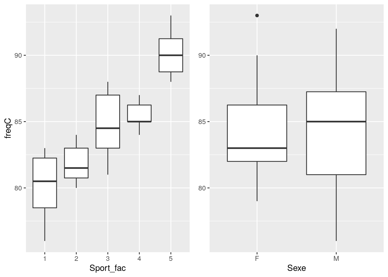
Anova 1 facteur
Question : ``Y a-t-il un effet de la pratique sportive sur la frequence cardiaque au repos ?’’
Ajustement du modèle :
Estimation et test sur les paramètres
##
## Call:
## lm(formula = freqC ~ Sport, data = freq)
##
## Residuals:
##     Min      1Q  Median      3Q     Max
## -3.7000 -1.5438 -0.1375  1.6125  3.8000
##
## Coefficients:
##             Estimate Std. Error t value Pr(>|t|)
## (Intercept)  77.3250     0.7719  100.18  < 2e-16 ***
## Sport         2.3750     0.2327   10.21 1.94e-12 ***
## ---
## Signif. codes:  0 '***' 0.001 '**' 0.01 '*' 0.05 '.' 0.1 ' ' 1
##
## Residual standard error: 2.082 on 38 degrees of freedom
## Multiple R-squared:  0.7327, Adjusted R-squared:  0.7256
## F-statistic: 104.1 on 1 and 38 DF,  p-value: 1.936e-12
Oh mais ça n’est pas une analyse de variance. Quelle andouille j’ai oublié d’utiliser Sport_fac plutôt que Sport. Je recommence.
Ajustement du modèle :
Estimation et test sur les paramètres
##
## Call:
## lm(formula = freqC ~ Sport_fac, data = freq)
##
## Residuals:
##    Min     1Q Median     3Q    Max
## -4.125 -1.562 -0.125  1.500  3.250
##
## Coefficients:
##             Estimate Std. Error t value Pr(>|t|)
## (Intercept)   80.125      0.709 113.012  < 2e-16 ***
## Sport_fac2     1.625      1.003   1.621    0.114
## Sport_fac3     4.625      1.003   4.613 5.14e-05 ***
## Sport_fac4     5.375      1.003   5.361 5.38e-06 ***
## Sport_fac5    10.000      1.003   9.973 9.09e-12 ***
## ---
## Signif. codes:  0 '***' 0.001 '**' 0.01 '*' 0.05 '.' 0.1 ' ' 1
##
## Residual standard error: 2.005 on 35 degrees of freedom
## Multiple R-squared:  0.7715, Adjusted R-squared:  0.7454
## F-statistic: 29.54 on 4 and 35 DF,  p-value: 8.766e-11
La matrice de design
##    (Intercept) Sport_fac2 Sport_fac3 Sport_fac4 Sport_fac5
## 1            1          0          0          0          0
## 2            1          0          0          0          0
## 3            1          0          0          0          0
## 4            1          0          0          0          0
## 5            1          0          0          0          0
## 6            1          0          0          0          0
## 7            1          0          0          0          0
## 8            1          0          0          0          0
## 9            1          1          0          0          0
## 10           1          1          0          0          0
## 11           1          1          0          0          0
## 12           1          1          0          0          0
## 13           1          1          0          0          0
## 14           1          1          0          0          0
## 15           1          1          0          0          0
## 16           1          1          0          0          0
## 17           1          0          1          0          0
## 18           1          0          1          0          0
## 19           1          0          1          0          0
## 20           1          0          1          0          0
## 21           1          0          1          0          0
## 22           1          0          1          0          0
## 23           1          0          1          0          0
## 24           1          0          1          0          0
## 25           1          0          0          1          0
## 26           1          0          0          1          0
## 27           1          0          0          1          0
## 28           1          0          0          1          0
## 29           1          0          0          1          0
## 30           1          0          0          1          0
## 31           1          0          0          1          0
## 32           1          0          0          1          0
## 33           1          0          0          0          1
## 34           1          0          0          0          1
## 35           1          0          0          0          1
## 36           1          0          0          0          1
## 37           1          0          0          0          1
## 38           1          0          0          0          1
## 39           1          0          0          0          1
## 40           1          0          0          0          1
## attr(,"assign")
## [1] 0 1 1 1 1
## attr(,"contrasts")
## attr(,"contrasts")$Sport_fac
## [1] "contr.treatment"
Dans le modèle linéaire \(Y=X\theta +E\), l’estimation des paramètres est donnée par
\[ \hat{\theta} = (X^\prime X )^{-1} X^\prime Y.\]
On peut retrouver les valeurs estimées sur cet exemple
Y <- matrix(freq$freqC, ncol = 1)
X <- model.matrix(lm_1)
Xprime <- t(X)

solve(Xprime %*% X) %*%  Xprime %*% Y
## [,1]
## (Intercept) 80.125
## Sport_fac2 1.625
## Sport_fac3 4.625
## Sport_fac4 5.375
## Sport_fac5 10.000La loi de l’estimateur \(T\) correspondant est donné par
\[T\sim\mathcal{N}\left( \theta, \sigma^2 (X^\prime X)^{-1} \right)\]
Test de l’effet global du niveau d’activité sportive .
## Analysis of Variance Table
##
## Response: freqC
##           Df Sum Sq Mean Sq F value    Pr(>F)
## Sport_fac  4 475.15 118.788  29.539 8.766e-11 ***
## Residuals 35 140.75   4.021
## ---
## Signif. codes: 0 '***' 0.001 '**' 0.01 '*' 0.05 '.' 0.1 ' ' 1## Analysis of Variance Table
##
## Model 1: freqC ~ 1
## Model 2: freqC ~ Sport_fac
## Res.Df RSS Df Sum of Sq F Pr(>F)
## 1 39 615.90
## 2 35 140.75 4 475.15 29.539 8.766e-11 ***
## ---
## Signif. codes: 0 '***' 0.001 '**' 0.01 '*' 0.05 '.' 0.1 ' ' 1## Analysis of Variance Table
##
## Response: freqC
## Df Sum Sq Mean Sq F value Pr(>F)
## Sport_fac 4 475.15 118.788 29.539 8.766e-11 ***
## Residuals 35 140.75 4.021
## ---
## Signif. codes: 0 '***' 0.001 '**' 0.01 '*' 0.05 '.' 0.1 ' ' 1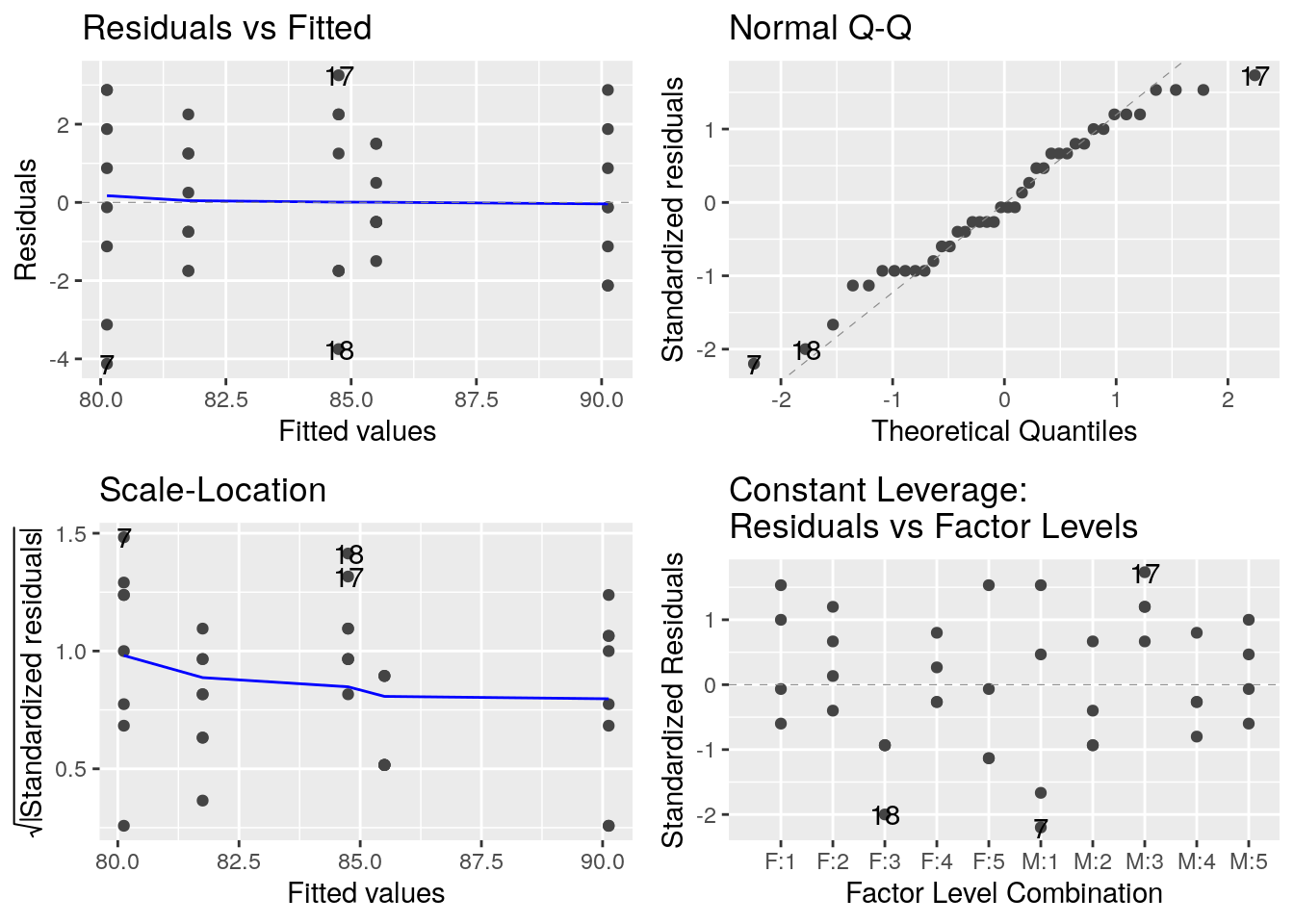
Anova deux facteurs, plan équilibré
Question : ``Y a-t-il un effet de la pratique sportive ou du sexe sur la frequence cardiaque au repos ?’’
Etude des interactions
freq %>%
  ggplot() +
  aes(x = Sport_fac, color = Sexe, group = Sexe, y = freqC) +
  stat_summary(fun.y = mean, geom = "point") +
  stat_summary(fun.y = mean, geom = "line")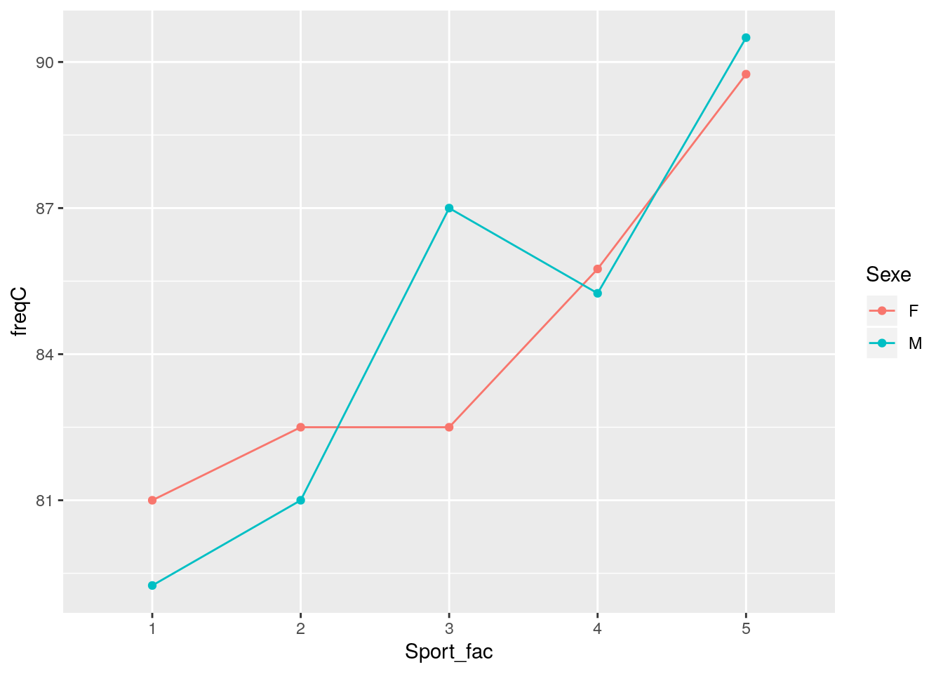
Modèle avec interaction :
##
## Call:
## lm(formula = freqC ~ Sexe + Sport + Sexe * Sport, data = freq)
##
## Residuals:
##    Min     1Q Median     3Q    Max
## -3.300 -1.319 -0.325  1.600  4.550
##
## Coefficients:
##             Estimate Std. Error t value Pr(>|t|)
## (Intercept)  78.0750     1.0936  71.395  < 2e-16 ***
## SexeM        -1.5000     1.5465  -0.970    0.339
## Sport         2.0750     0.3297   6.293 2.82e-07 ***
## SexeM:Sport   0.6000     0.4663   1.287    0.206
## ---
## Signif. codes:  0 '***' 0.001 '**' 0.01 '*' 0.05 '.' 0.1 ' ' 1
##
## Residual standard error: 2.085 on 36 degrees of freedom
## Multiple R-squared:  0.7458, Adjusted R-squared:  0.7246
## F-statistic: 35.21 on 3 and 36 DF, p-value: 8.35e-11##
## Call:
## lm(formula = freqC ~ Sexe + Sport_fac + Sexe * Sport_fac, data = freq)
##
## Residuals:
## Min 1Q Median 3Q Max
## -3.25 -1.00 0.00 1.00 3.75
##
## Coefficients:
## Estimate Std. Error t value Pr(>|t|)
## (Intercept) 81.0000 0.8563 94.588 < 2e-16 ***
## SexeM -1.7500 1.2111 -1.445 0.158819
## Sport_fac2 1.5000 1.2111 1.239 0.225104
## Sport_fac3 1.5000 1.2111 1.239 0.225104
## Sport_fac4 4.7500 1.2111 3.922 0.000473 ***
## Sport_fac5 8.7500 1.2111 7.225 4.84e-08 ***
## SexeM:Sport_fac2 0.2500 1.7127 0.146 0.884923
## SexeM:Sport_fac3 6.2500 1.7127 3.649 0.000991 ***
## SexeM:Sport_fac4 1.2500 1.7127 0.730 0.471147
## SexeM:Sport_fac5 2.5000 1.7127 1.460 0.154770
## ---
## Signif. codes: 0 '***' 0.001 '**' 0.01 '*' 0.05 '.' 0.1 ' ' 1
##
## Residual standard error: 1.713 on 30 degrees of freedom
## Multiple R-squared: 0.8571, Adjusted R-squared: 0.8143
## F-statistic: 20 on 9 and 30 DF, p-value: 2.327e-10Test du modèle complet

## Analysis of Variance Table
##
## Model 1: freqC ~ 1
## Model 2: freqC ~ Sexe + Sport_fac + Sexe * Sport_fac
##   Res.Df   RSS Df Sum of Sq      F    Pr(>F)
## 1     39 615.9
## 2     30  88.0  9     527.9 19.996 2.327e-10 ***
## ---
## Signif. codes: 0 '***' 0.001 '**' 0.01 '*' 0.05 '.' 0.1 ' ' 1- Question : ``Y a-t-il un effet de la pratique sportive sur la fréquence cardiaque au repos ?’’ \
Question : ``Y a-t-il un effet du sexe sur la fréquence cardiaque au repos ?’’
Question : ``Y a-t-il un effet du sexe en interaction avec la pratique sportive sur la fréquence cardiaque au repos ?’’
On commence toujours par tester l’effet de l’interaction.
## Analysis of Variance Table
##
## Model 1: freqC ~ Sport_fac + Sexe
## Model 2: freqC ~ Sexe + Sport_fac + Sexe * Sport_fac
##   Res.Df    RSS Df Sum of Sq     F   Pr(>F)
## 1     34 139.85
## 2     30  88.00  4     51.85 4.419 0.006299 **
## ---
## Signif. codes: 0 '***' 0.001 '**' 0.01 '*' 0.05 '.' 0.1 ' ' 1## Analysis of Variance Table
##
## Response: freqC
## Df Sum Sq Mean Sq F value Pr(>F)
## Sexe 1 0.90 0.900 0.3068 0.583745
## Sport_fac 4 475.15 118.787 40.4957 1.105e-11 ***
## Sexe:Sport_fac 4 51.85 12.962 4.4190 0.006299 **
## Residuals 30 88.00 2.933
## ---
## Signif. codes: 0 '***' 0.001 '**' 0.01 '*' 0.05 '.' 0.1 ' ' 1## Anova Table (Type II tests)
##
## Response: freqC
## Sum Sq Df F value Pr(>F)
## Sexe 0.90 1 0.3068 0.583745
## Sport_fac 475.15 4 40.4957 1.105e-11 ***
## Sexe:Sport_fac 51.85 4 4.4190 0.006299 **
## Residuals 88.00 30
## ---
## Signif. codes: 0 '***' 0.001 '**' 0.01 '*' 0.05 '.' 0.1 ' ' 1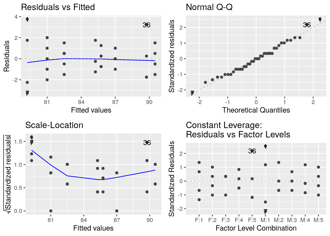
Modèle sans interaction :
##
## Call:
## lm(formula = freqC ~ Sexe + Sport_fac, data = freq)
##
## Residuals:
##    Min     1Q Median     3Q    Max
## -4.275 -1.600 -0.125  1.462  3.100
##
## Coefficients:
##             Estimate Std. Error t value Pr(>|t|)
## (Intercept)  79.9750     0.7855 101.816  < 2e-16 ***
## SexeM         0.3000     0.6413   0.468    0.643
## Sport_fac2    1.6250     1.0141   1.602    0.118
## Sport_fac3    4.6250     1.0141   4.561 6.32e-05 ***
## Sport_fac4    5.3750     1.0141   5.300 6.99e-06 ***
## Sport_fac5   10.0000     1.0141   9.861 1.67e-11 ***
## ---
## Signif. codes:  0 '***' 0.001 '**' 0.01 '*' 0.05 '.' 0.1 ' ' 1
##
## Residual standard error: 2.028 on 34 degrees of freedom
## Multiple R-squared:  0.7729, Adjusted R-squared:  0.7395
## F-statistic: 23.15 on 5 and 34 DF,  p-value: 4.63e-10
Question : Y a-t-il un effet de la pratique sportive sur la fréquence cardiaque au repos ?''\\ Question :Y a-t-il un effet du sexe sur la fréquence cardiaque au repos ?’’
## Analysis of Variance Table
##
## Response: freqC
##           Df Sum Sq Mean Sq F value    Pr(>F)
## Sexe       1   0.90   0.900  0.2188    0.6429
## Sport_fac  4 475.15 118.787 28.8793 1.643e-10 ***
## Residuals 34 139.85   4.113
## ---
## Signif. codes: 0 '***' 0.001 '**' 0.01 '*' 0.05 '.' 0.1 ' ' 1## Anova Table (Type II tests)
##
## Response: freqC
## Sum Sq Df F value Pr(>F)
## Sexe 0.90 1 0.2188 0.6429
## Sport_fac 475.15 4 28.8793 1.643e-10 ***
## Residuals 139.85 34
## ---
## Signif. codes: 0 '***' 0.001 '**' 0.01 '*' 0.05 '.' 0.1 ' ' 1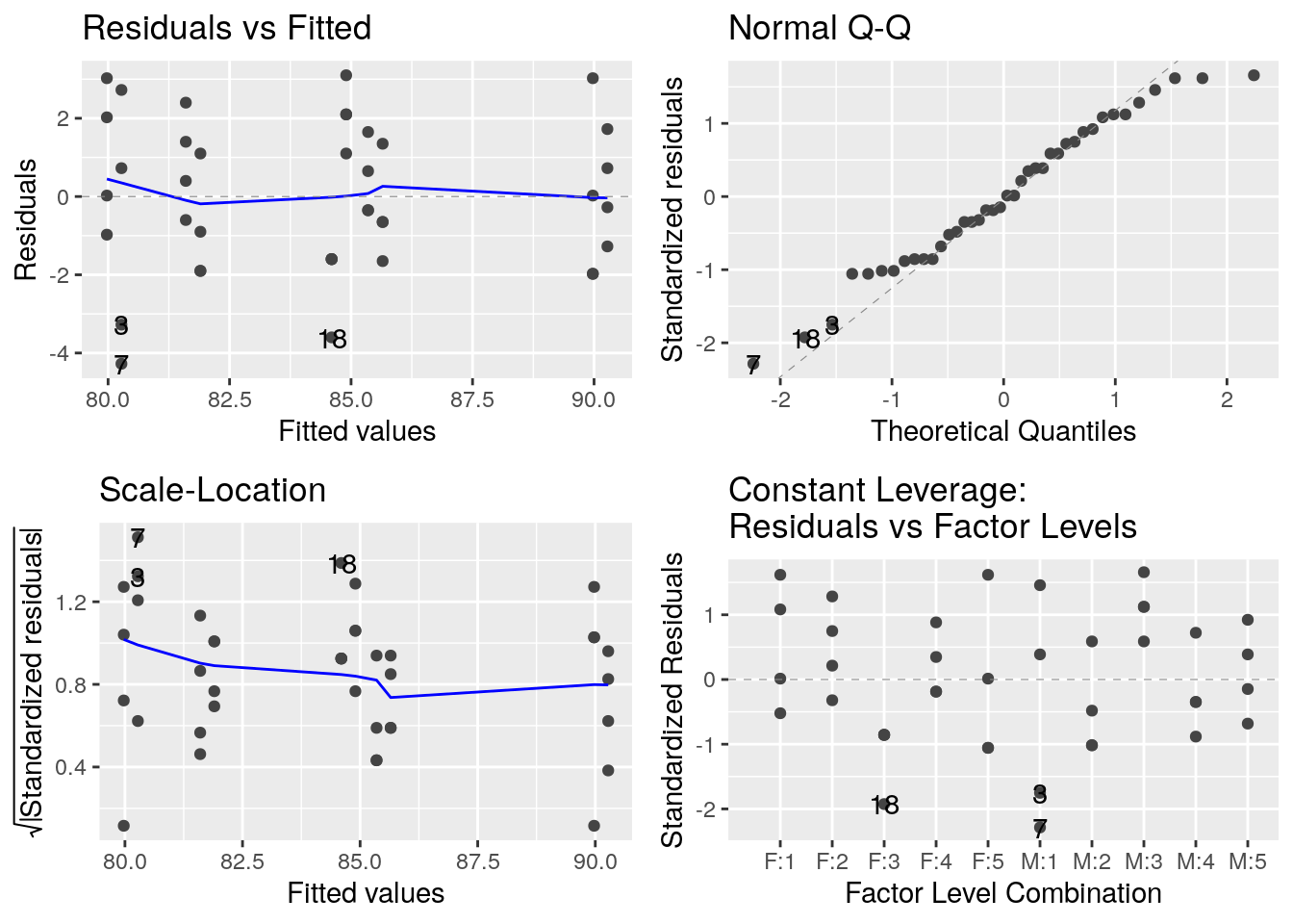
Anova deux facteurs, plan déséquilibré
 freq2 <- read.table(file = "data/FreqCardiaqueDes1.txt", header = T)
freq2 <- freq2 %>% mutate(Sport_fac = as.factor(Sport))
table(freq2$Sexe, freq2$Sport)
##
## 1 2 3 4 5
## F 6 3 5 3 2
## M 3 2 6 5 5## # A tibble: 10 x 3
## Sport Sexe n
## <int> <fct> <int>
## 1 1 F 6
## 2 1 M 3
## 3 2 F 3
## 4 2 M 2
## 5 3 F 5
## 6 3 M 6
## 7 4 F 3
## 8 4 M 5
## 9 5 F 2
## 10 5 M 5Moyennes et écart-types par groupes :
## # A tibble: 5 x 2
##   Sport mean_freq
##   <int>     <dbl>
## 1     1      80.6
## 2     2      81.8
## 3     3      85.4
## 4     4      85.4
## 5 5 91.3## # A tibble: 2 x 2
## Sexe mean_freq
## <fct> <dbl>
## 1 F 83.7
## 2 M 85.9## # A tibble: 10 x 3
## # Groups: Sport [5]
## Sport Sexe mean_freq
## <int> <fct> <dbl>
## 1 1 F 80.7
## 2 1 M 80.3
## 3 2 F 83
## 4 2 M 80
## 5 3 F 83
## 6 3 M 87.3
## 7 4 F 85.7
## 8 4 M 85.2
## 9 5 F 93
## 10 5 M 90.6p1 <- ggplot(freq2, aes(y=freqC, x = Sport_fac)) + geom_boxplot()
p2 <- ggplot(freq2, aes(y=freqC, x = Sexe)) + geom_boxplot()
ggarrange(p1,p2+rremove('ylab'))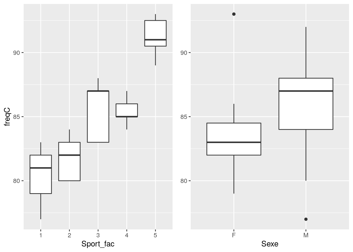
freq2 %>%
  ggplot() +
  aes(x = Sport_fac, color = Sexe, group = Sexe, y = freqC) +
  stat_summary(fun.y = mean, geom = "point") +
  stat_summary(fun.y = mean, geom = "line")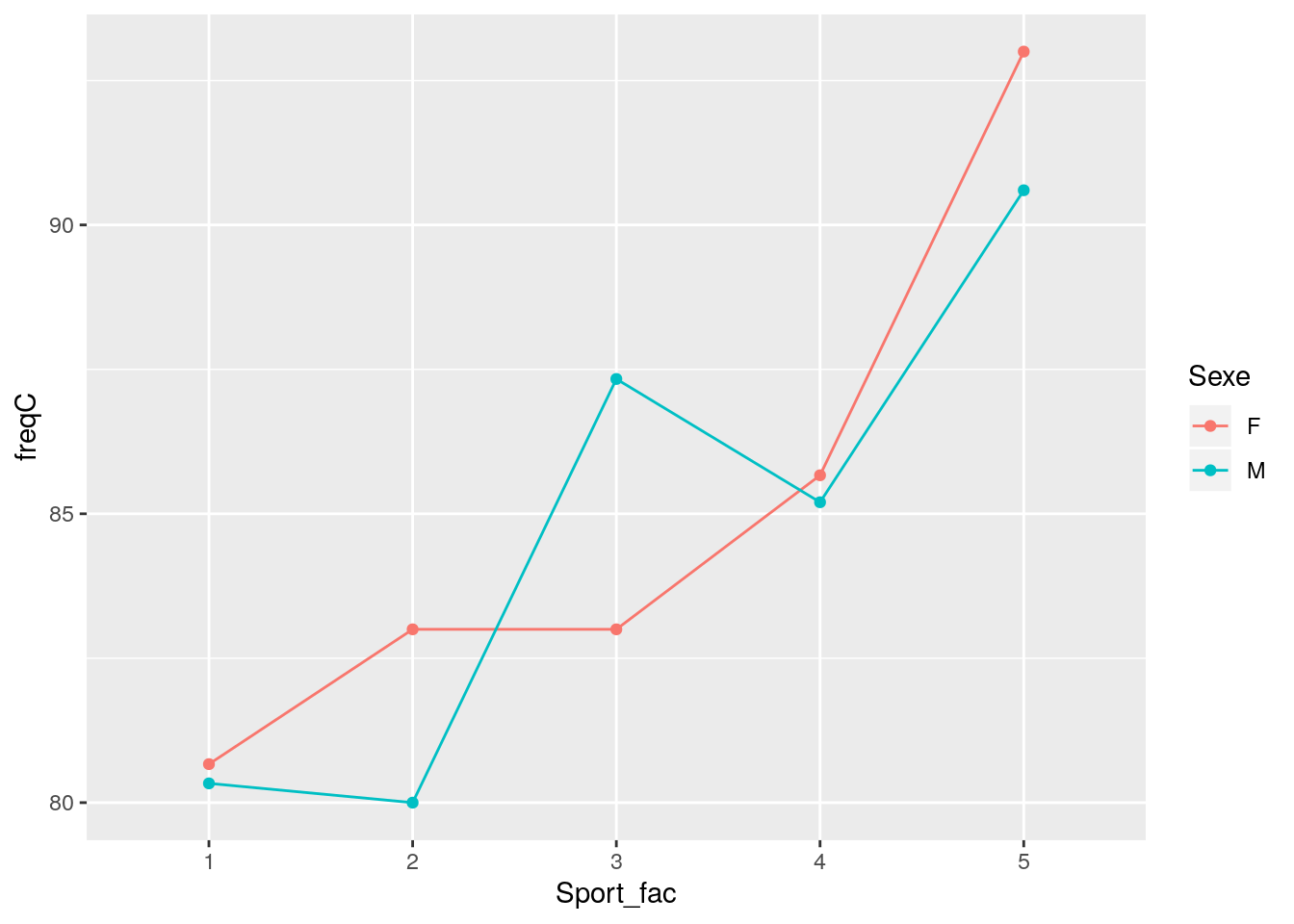
## Analysis of Variance Table
##
## Response: freqC
##                Df Sum Sq Mean Sq F value    Pr(>F)
## Sport_fac       4 507.50 126.876 76.1256 2.863e-15 ***
## Sexe            1   1.14   1.143  0.6857    0.4142
## Sport_fac:Sexe  4  69.73  17.432 10.4593 1.995e-05 ***
## Residuals      30  50.00   1.667
## ---
## Signif. codes: 0 '***' 0.001 '**' 0.01 '*' 0.05 '.' 0.1 ' ' 1## Anova Table (Type II tests)
##
## Response: freqC
## Sum Sq Df F value Pr(>F)
## Sport_fac 461.77 4 69.2648 1.025e-14 ***
## Sexe 1.14 1 0.6857 0.4142
## Sport_fac:Sexe 69.73 4 10.4593 1.995e-05 ***
## Residuals 50.00 30
## ---
## Signif. codes: 0 '***' 0.001 '**' 0.01 '*' 0.05 '.' 0.1 ' ' 1On change l’ordre des facteurs

## Analysis of Variance Table
##
## Response: freqC
##                Df Sum Sq Mean Sq F value    Pr(>F)
## Sport_fac       4 507.50 126.876 76.1256 2.863e-15 ***
## Sexe            1   1.14   1.143  0.6857    0.4142
## Sport_fac:Sexe  4  69.73  17.432 10.4593 1.995e-05 ***
## Residuals      30  50.00   1.667
## ---
## Signif. codes: 0 '***' 0.001 '**' 0.01 '*' 0.05 '.' 0.1 ' ' 1## NOTE: Results may be misleading due to involvement in interactions## $emmeans
## Sport_fac emmean SE df lower.CL upper.CL
## 1 80.5 0.456 30 79.6 81.4
## 2 81.5 0.589 30 80.3 82.7
## 3 85.2 0.391 30 84.4 86.0
## 4 85.4 0.471 30 84.5 86.4
## 5 91.8 0.540 30 90.7 92.9
##
## Results are averaged over the levels of: Sexe
## Confidence level used: 0.95
##
## $contrasts
## contrast estimate SE df t.ratio p.value
## 1 - 2 -1.000 0.745 30 -1.342 0.3796
## 1 - 3 -4.667 0.601 30 -7.766 <.0001
## 1 - 4 -4.933 0.656 30 -7.518 <.0001
## 1 - 5 -11.300 0.707 30 -15.981 <.0001
## 2 - 3 -3.667 0.707 30 -5.185 <.0001
## 2 - 4 -3.933 0.755 30 -5.212 <.0001
## 2 - 5 -10.300 0.799 30 -12.886 <.0001
## 3 - 4 -0.267 0.612 30 -0.435 0.6663
## 3 - 5 -6.633 0.667 30 -9.950 <.0001
## 4 - 5 -6.367 0.717 30 -8.881 <.0001
##
## Results are averaged over the levels of: Sexe
## P value adjustment: hochberg method for 10 tests