Présentation
Ce premier TD vise à explorer les données spatialisées de précipitations en Suisse. Nous utiliserons R et plusieurs packages spécialisés (tidyverse, sf, gstat, etc.) pour visualiser, analyser et modéliser ces données.
Utilisez les clusters cluster1 et cluster2
Objectifs
Charger et visualiser les données spatialisées.
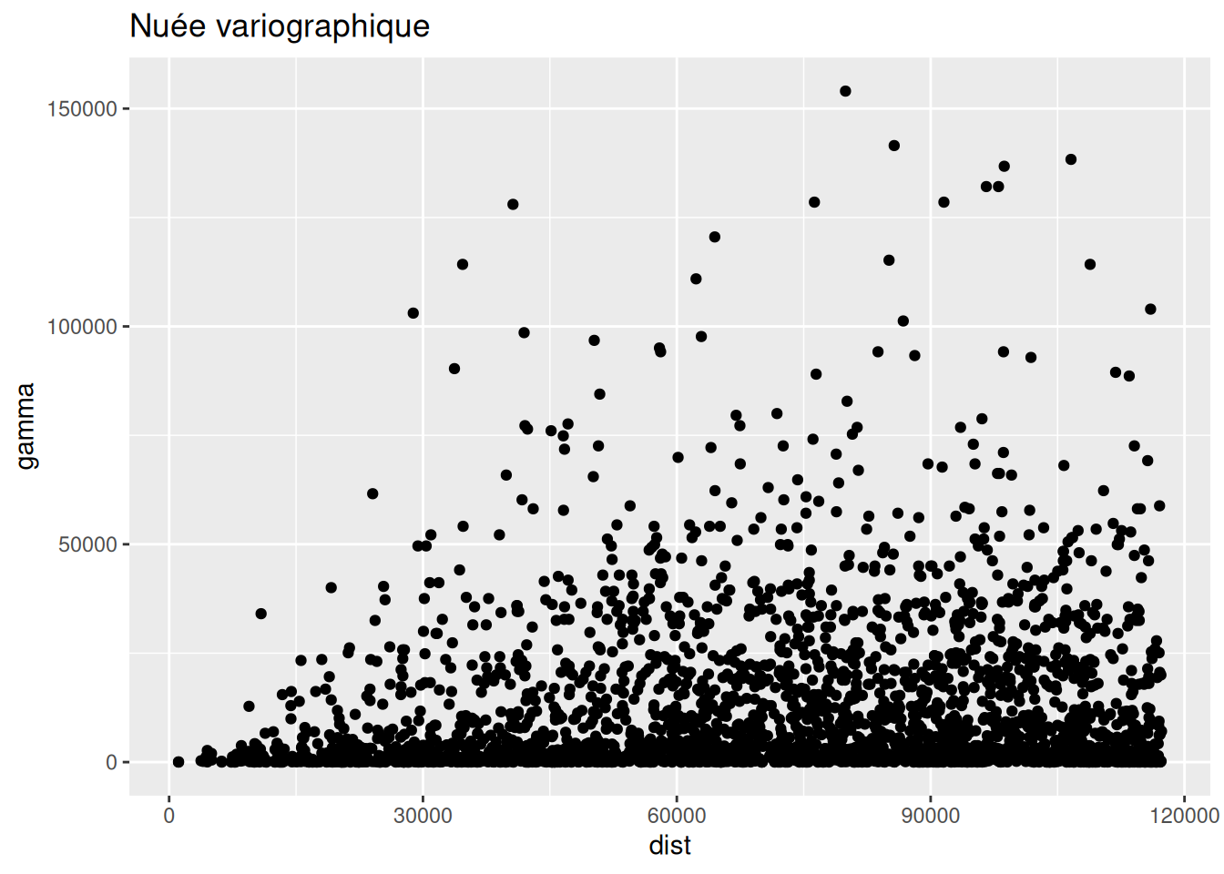
Construire et interpréter des nuées variographiques.
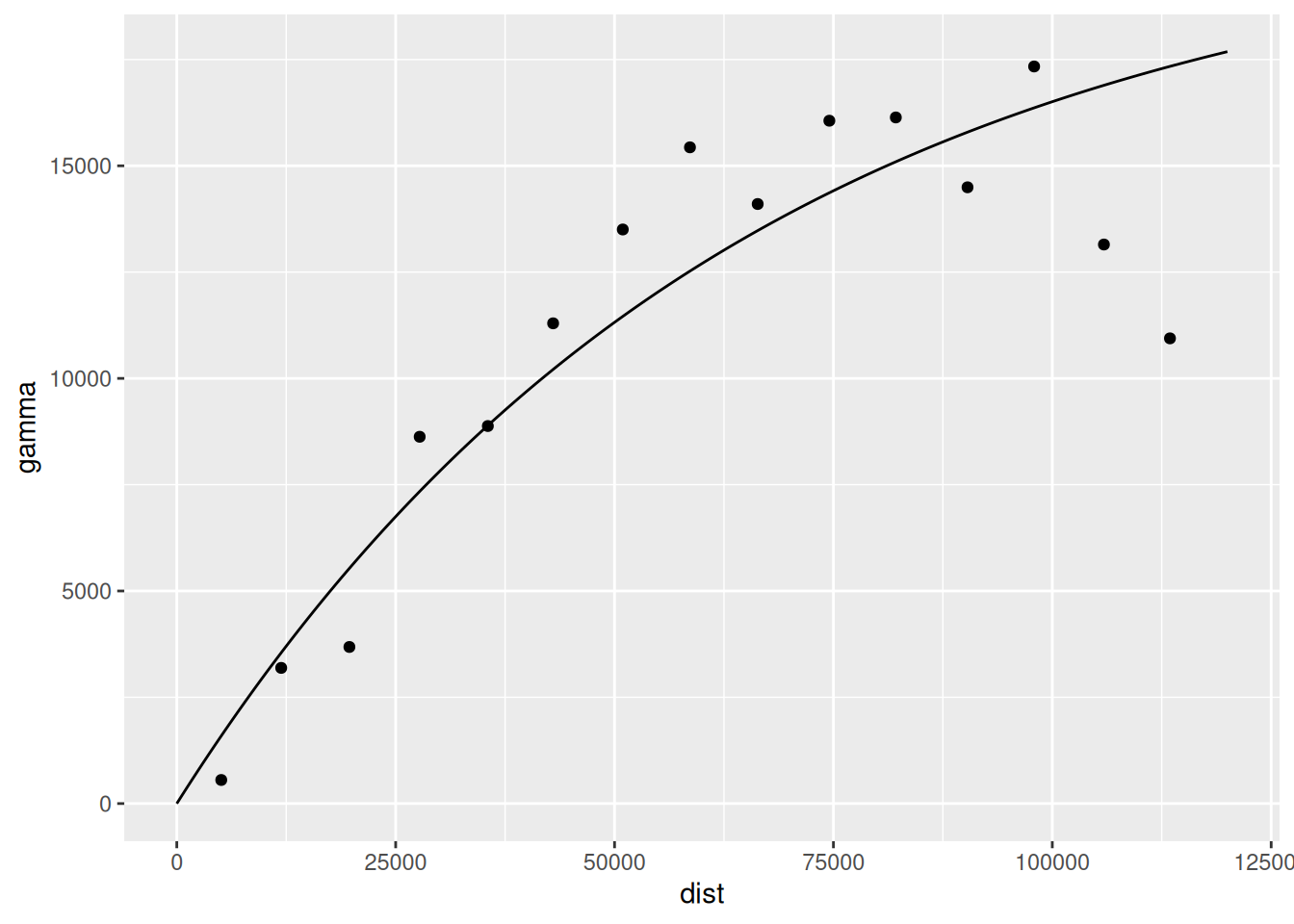
Estimer et ajuster des variogrammes.
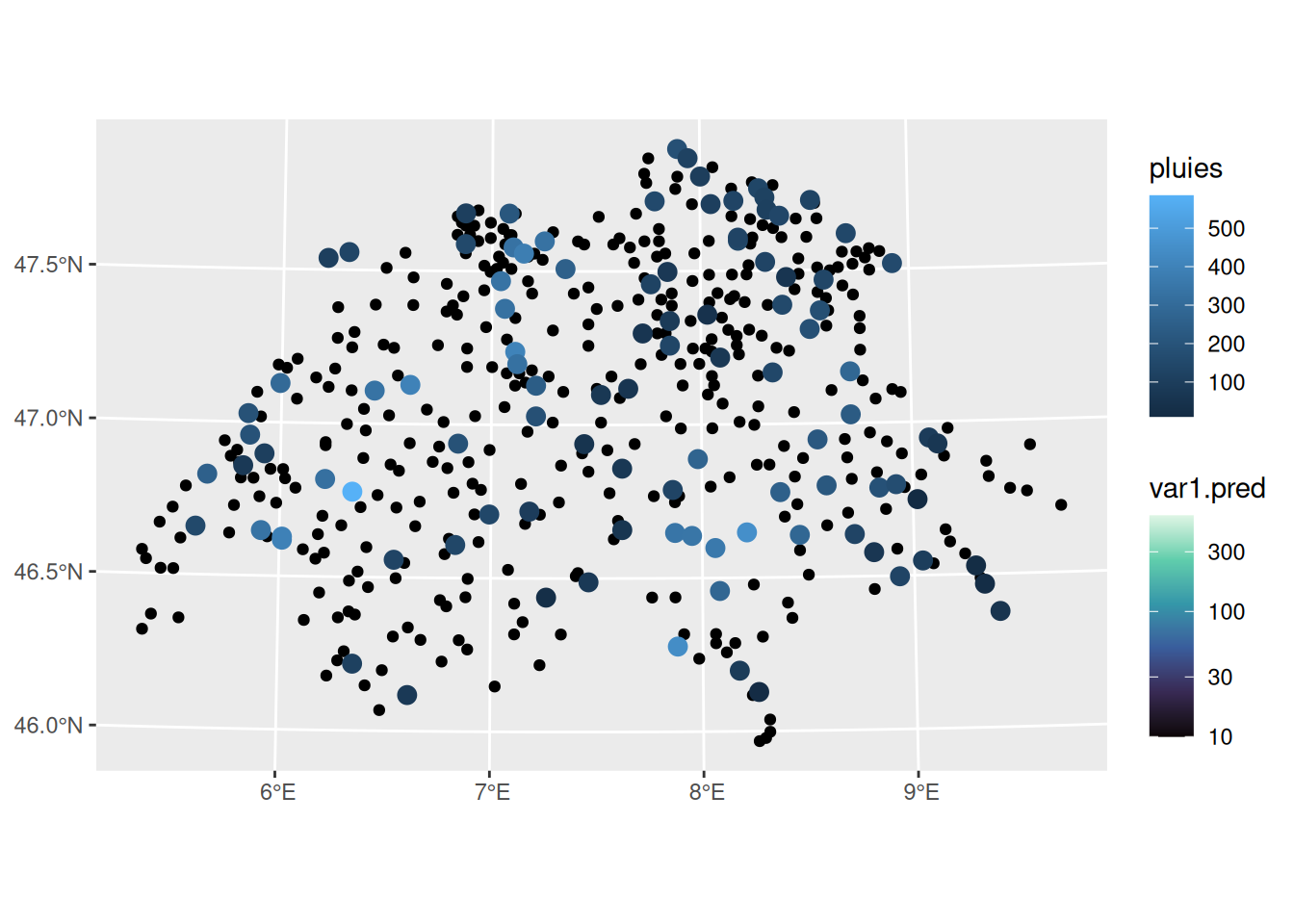
Effectuer un krigeage pour interpoler les précipitations.
Tester différentes structures de variogramme et intégrer une covariable.
Directives
1. Chargement et visualisation des données
── Attaching core tidyverse packages ──────────────────────── tidyverse 2.0.0 ──
✔ dplyr     1.2.1     ✔ readr     2.2.0
✔ forcats   1.0.1     ✔ stringr   1.6.0
✔ ggplot2   4.0.3     ✔ tibble    3.3.1
✔ lubridate 1.9.5     ✔ tidyr     1.3.2
✔ purrr     1.2.2
── Conflicts ────────────────────────────────────────── tidyverse_conflicts() ──
✖ dplyr::filter() masks stats::filter()
✖ dplyr::lag()    masks stats::lag()
ℹ Use the conflicted package (<http://conflicted.r-lib.org/>) to force all conflicts to become errors
library (ggforce)library (gstat)library (sf)
Linking to GEOS 3.14.1, GDAL 3.12.2, PROJ 9.7.1; sf_use_s2() is TRUE
<- st_read (dsn = "swiss/swiss_rain_full.shp" )
Reading layer `swiss_rain_full' from data source
  `/__w/statspat/statspat/swiss/swiss_rain_full.shp' using driver `ESRI Shapefile'
Simple feature collection with 467 features and 1 field
Geometry type: POINT
Dimension:     XY
Bounding box:  xmin: -159812 ymin: -109008 xmax: 172891 ymax: 105361
Projected CRS: CH1903 (Bern) / LV03C
<- st_read (dsn = "swiss/swiss_rain.shp" )
Reading layer `swiss_rain' from data source
  `/__w/statspat/statspat/swiss/swiss_rain.shp' using driver `ESRI Shapefile'
Simple feature collection with 100 features and 1 field
Geometry type: POINT
Dimension:     XY
Bounding box:  xmin: -140463 ymin: -92327 xmax: 150921 ymax: 105361
Projected CRS: CH1903 (Bern) / LV03C
<- st_read (dsn = "swiss/bords.shp" )
Reading layer `bords' from data source `/__w/statspat/statspat/swiss/bords.shp' using driver `ESRI Shapefile'
Simple feature collection with 1 feature and 1 field
Geometry type: POLYGON
Dimension:     XY
Bounding box:  xmin: -169990 ymin: -111696 xmax: 177126 ymax: 108158
Projected CRS: CH1903 (Bern) / LV03C
<- st_read (dsn = "swiss/elev.shp" )
Reading layer `elev' from data source `/__w/statspat/statspat/swiss/elev.shp' using driver `ESRI Shapefile'
Simple feature collection with 95128 features and 1 field
Geometry type: POINT
Dimension:     XY
Bounding box:  xmin: -185556.4 ymin: -127261.5 xmax: 193184.2 ymax: 127252.2
Projected CRS: CH1903 (Bern) / LV03C
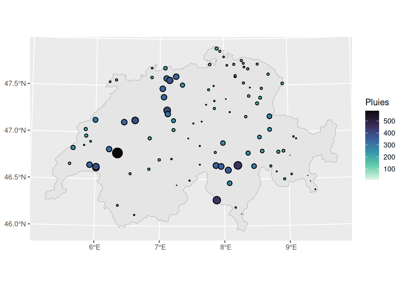
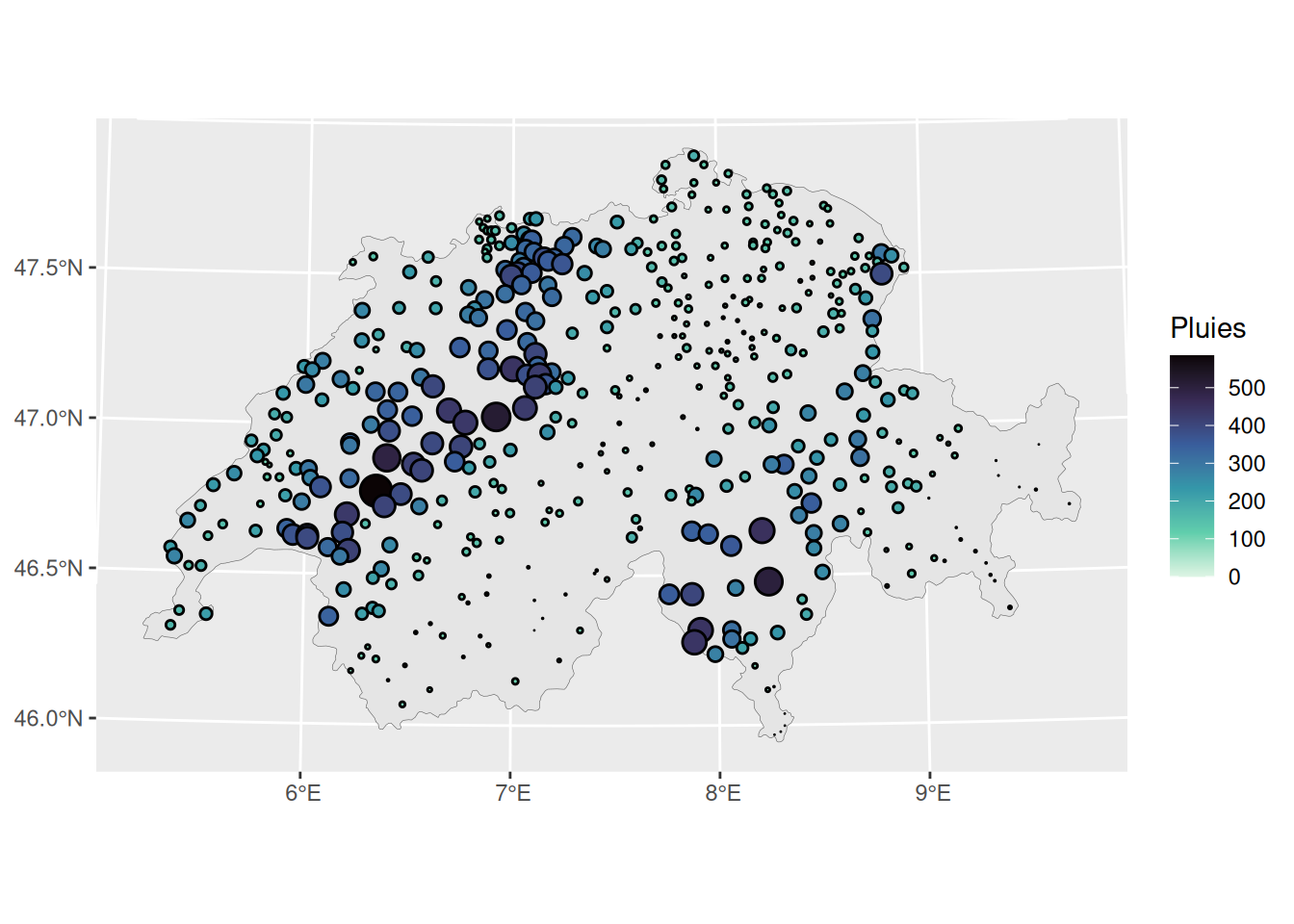
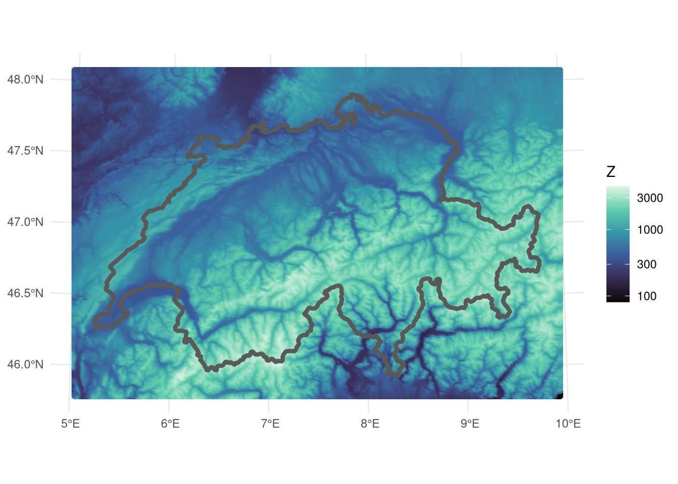
|> st_coordinates () |> bind_cols (dta_sf) |> ggplot () + geom_sf (data = bords_sf, linewidth = 0.1 ) + geom_circle (aes (x0= X, y0= Y, r= pluies* 10 , fill = pluies)) + scale_fill_viridis_c (name = "Pluies" , option = "mako" , direction = - 1 ) |> st_coordinates () |> bind_cols (dta_full_sf) |> ggplot () + geom_sf (data = bords_sf, linewidth = 0.1 ) + geom_circle (aes (x0= X, y0= Y, r= pluies* 10 , fill = pluies)) + scale_fill_viridis_c (name = "Pluies" , option = "mako" , direction = - 1 ) |> ggplot () + geom_sf (aes (col = elevation)) + geom_sf (data = bords_sf, fill = NA , linewidth = 1.5 ) + theme_minimal () + theme (legend.position = "right" ) + scale_color_viridis_c (name = "Z" , option = "mako" , transform= "log10" )
2. Nuées variographiques à la main
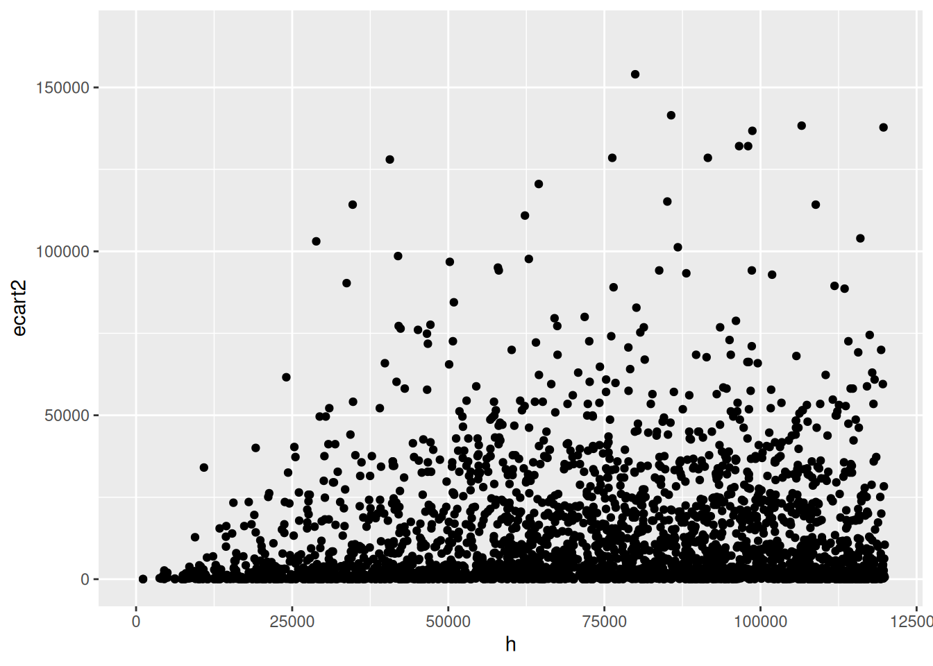
<- do.call (rbind, lapply (1 : nrow (dta_sf), function (i) {<- st_coordinates (dta_sf)<- xy[i, 1 ]<- xy[i, 2 ]<- dta_sf$ pluies[i]|> rownames_to_column ('Id' ) |> mutate (delta_x = xy[,1 ] - x0, delta_y = xy[,2 ] - y0, ecart = pluies - pluie0) |> filter (Id > i) |> mutate (h = sqrt (delta_x^ 2 + delta_y^ 2 ), ecart2 = ecart^ 2 / 2 ) |> select (Id, h, ecart2)|> ggplot () + geom_point (aes (x= h, y= ecart2)) + xlim (c (0 , 120000 ))
Warning: Removed 2125 rows containing missing values or values outside the scale range
(`geom_point()`).
3. Variogramme empirique
<- variogram (pluies~ 1 , data = dta_sf, cloud = TRUE )|> ggplot (aes (x= dist, y= gamma)) + geom_point () + ggtitle ("Nuée variographique" )
4. Ajustement du variogramme
<- variogram (pluies~ 1 , data = dta_sf)<- fit.variogram (vario.iso, vgm (model = "Exp" , psill = 90000 , range = 50000 ))<- variogramLine (v.fit, maxdist = 120000 )ggplot (data = vario.iso, aes (x= dist, y= gamma)) + geom_point () + geom_line (data= vario_fit_exp , aes (x= dist, y= gamma))
5. Krigeage
<- krige (formula = pluies ~ 1 , locations = dta_sf, newdata = dta_full_sf, model = v.fit)
Registered S3 method overwritten by 'stars':
  method                  from
  st_interpolate_aw.stars sf
|> ggplot () + geom_sf (aes (fill = var1.pred)) + geom_sf (data = dta_sf, aes (col = pluies), size= 3 ) + scale_fill_viridis_c (option = "mako" , transform = "log10" )
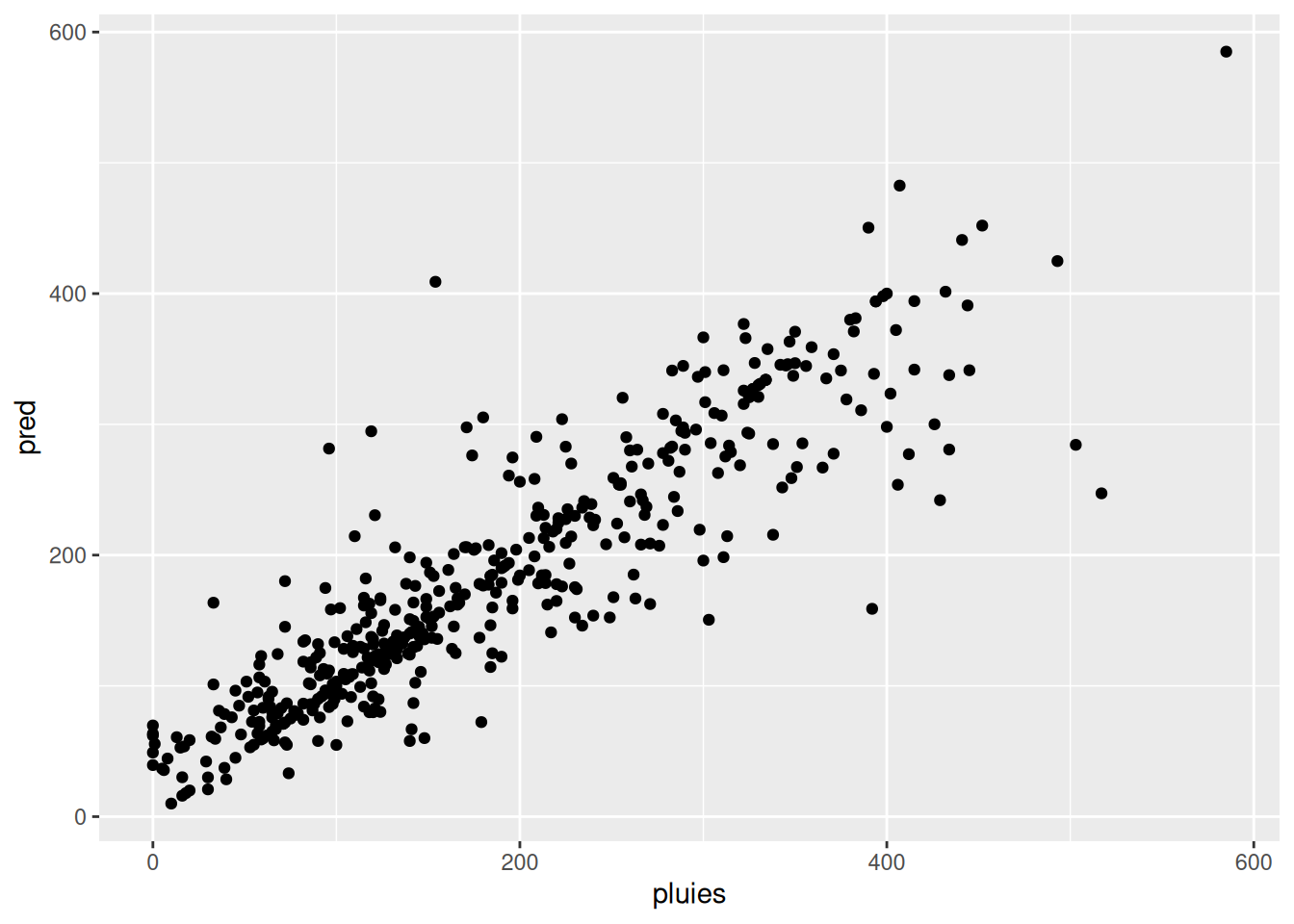
Prédites en fonction des observées
<- data.frame (pred = Kfull$ var1.pred)|> mutate (pred = Kfull$ var1.pred) |> ggplot () + geom_point (aes (x= pluies, y = pred))
6. À votre tour
Tester différentes formes de variogramme (exponentiel, gaussien, sphérique).
Ajouter une covariable (altitude) au modèle de krigeage et comparer les résultats.