TD3 : Modèles spatiaux et régression SAR

Analyse de la prédation au sein du golfe du Saint-Laurent

Author

Affiliation

Marie-Pierre Etienne

https://marieetienne.github.io/statspat

Pêches et Océans Canada conduit chaque année des campagnes de suivi dans le Golf du Saint Laurent. Le plan de suivi est construit à partir d’une stratification du golfe (strates spatiales construites pour avoir des habitats relativement homogènes). Plusieurs mesures par strates sont faites et nous avons ici accès à la valeur vomyenne de ces mesures pour chaque strate.

Plus précisément, Les variables d’intérêt sont

• dans le fichier StLaurent.csv

  • totconsum : indice de prédation total,
  • depth : profondeur,
  • temperature : température,
  • BH : présence de Bernards-l’hermite, (pas utilisée ici)

• dans le répertoire strates_saint_laurent le fichier shapefile strates.shp contient les caractéristiques spatiales des strates administratives

Les packages utilisés seront

library(tidyverse)

── Attaching core tidyverse packages ──────────────────────── tidyverse 2.0.0 ──
✔ dplyr     1.1.4     ✔ readr     2.1.5
✔ forcats   1.0.0     ✔ stringr   1.5.1
✔ ggplot2   3.5.1     ✔ tibble    3.2.1
✔ lubridate 1.9.4     ✔ tidyr     1.3.1
✔ purrr     1.0.4     
── Conflicts ────────────────────────────────────────── tidyverse_conflicts() ──
✖ dplyr::filter() masks stats::filter()
✖ dplyr::lag()    masks stats::lag()
ℹ Use the conflicted package (<http://conflicted.r-lib.org/>) to force all conflicts to become errors

library(sf)

Linking to GEOS 3.12.1, GDAL 3.8.4, PROJ 9.4.0; sf_use_s2() is TRUE

library(spdep)

Loading required package: spData
To access larger datasets in this package, install the spDataLarge
package with: `install.packages('spDataLarge',
repos='https://nowosad.github.io/drat/', type='source')`

library(spatialreg)

Loading required package: Matrix

Attaching package: 'Matrix'

The following objects are masked from 'package:tidyr':

    expand, pack, unpack


Attaching package: 'spatialreg'

The following objects are masked from 'package:spdep':

    get.ClusterOption, get.coresOption, get.mcOption,
    get.VerboseOption, get.ZeroPolicyOption, set.ClusterOption,
    set.coresOption, set.mcOption, set.VerboseOption,
    set.ZeroPolicyOption

# library(GGally) #eventuellement pour des stats desc 
library(purrr) # pour la validation croisée

1. Les données

Les données peuvent être chargées avec

dta <- read.csv("StLaurent.csv", sep = ";") |> mutate(log_totconsum = log(totconsum))
 

strates_sf <- st_read("strates_saint_laurent/strates.shp")

Reading layer `strates' from data source 
  `/__w/statspat/statspat/strates_saint_laurent/strates.shp' 
  using driver `ESRI Shapefile'

Warning in CPL_read_ogr(dsn, layer, query, as.character(options), quiet, : GDAL
Message 1: /__w/statspat/statspat/strates_saint_laurent/strates.shp contains
polygon(s) with rings with invalid winding order. Autocorrecting them, but that
shapefile should be corrected using ogr2ogr for example.

Simple feature collection with 38 features and 1 field
Geometry type: MULTIPOLYGON
Dimension:     XY
Bounding box:  xmin: -65.9368 ymin: 45.6756 xmax: -60.0779 ymax: 49.17685
Geodetic CRS:  WGS 84

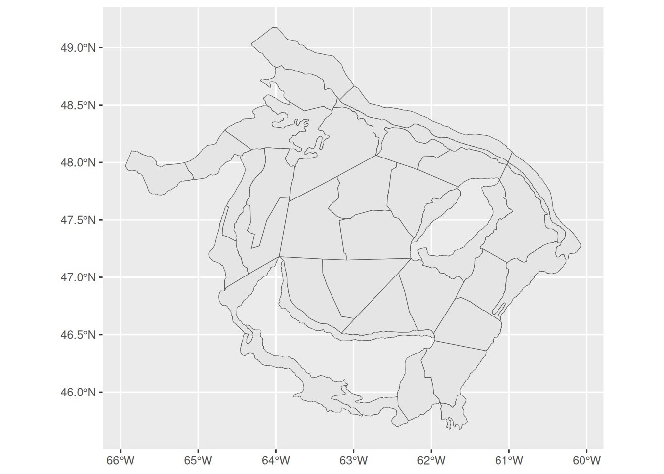
strates_sf |> ggplot() + geom_sf()

nrow(strates_sf)

[1] 38

1. Décrire les variables du tableau dta. Les classer par type (quantitatives, qualitatives, spatiales). Faire une analyse descriptive rapide des données.

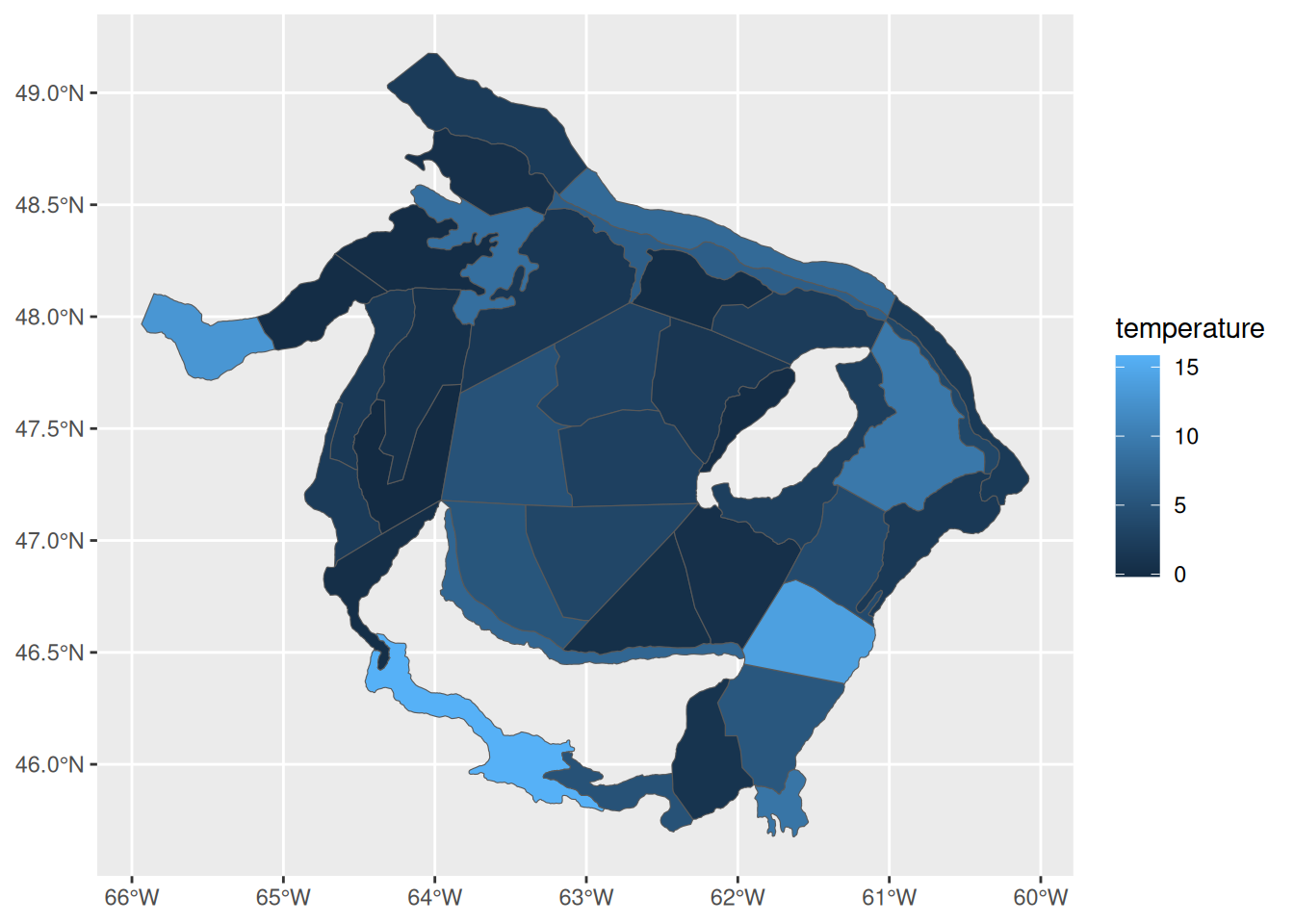
2. Mettre à jour la table strates_sf pour qu’elle contienne toutes les données et proposer une visualisation spatiale des données de température.

Joining with `by = join_by(strate)`

Warning in st_point_on_surface.sfc(sf::st_zm(x)): st_point_on_surface may not
give correct results for longitude/latitude data

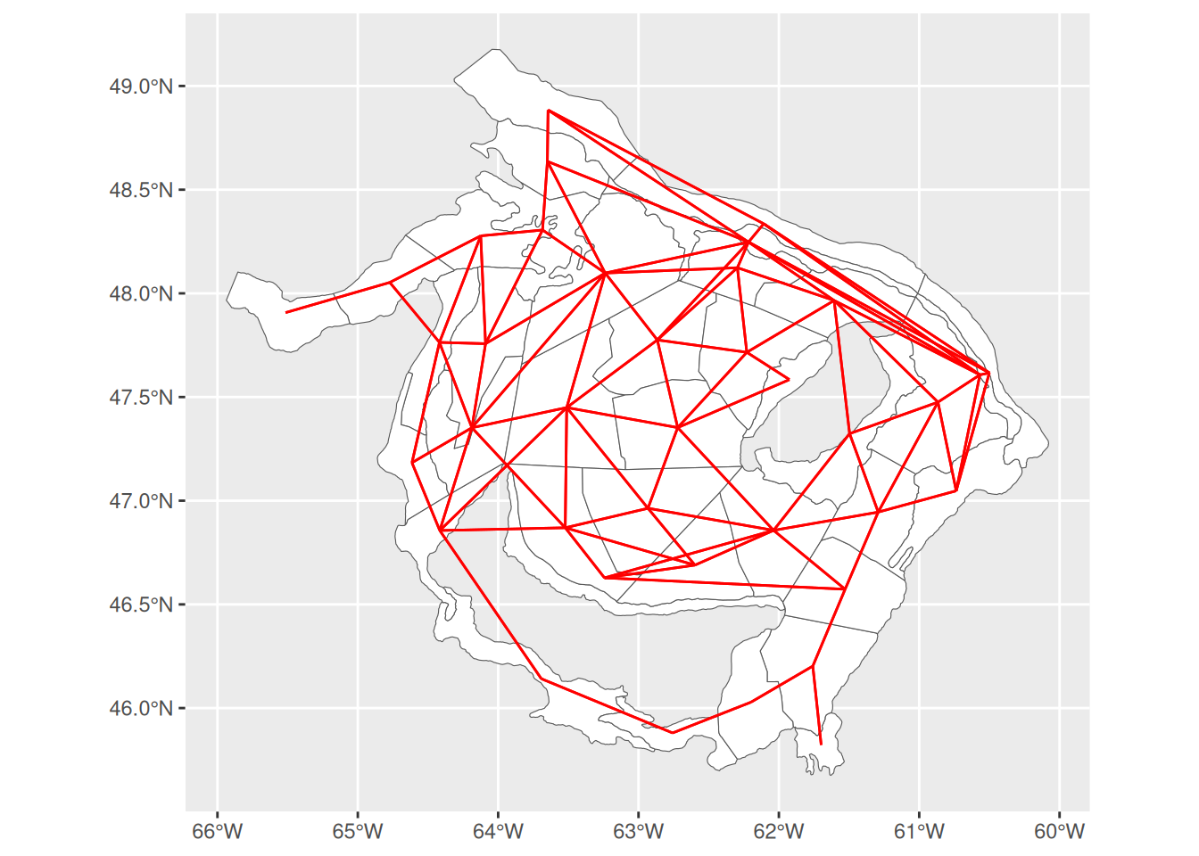
2. Systèmes de voisinage

Nous construisons plusieurs définitions de voisinage spatial.

centroids <- st_centroid(strates_sf)

Warning: st_centroid assumes attributes are constant over geometries

coords <- st_coordinates(centroids)

voisin_poly <- poly2nb(strates_sf)
ppv <- knearneigh(coords, k=4, longlat=TRUE)
voisin_knn4 <- knn2nb(ppv)
voisin_dm <- dnearneigh(as.matrix(coords), d1=0, d2=100, longlat=TRUE)

3. Expliquer les différences conceptuelles entre :

• voisinage par contiguïté de polygones (poly2nb),
• k plus proches voisins (knn2nb),
• distance maximale (dnearneigh).

4. Pourquoi le choix du voisinage influence-t-il les conclusions statistiques ?

Les fonctions pour construire les graphes de voisinage proviennent du package spdep et ne sont pas directement au format sf la fonction ci-dessous va nous permettre de représenter en format sf le graphe de voisinage associé à un système de voisinage.

nb_to_sflines <- function(nb, coords, crs = NA) {
  # nb    : object of class "nb"
  # coords: matrix n x 2 (usually st_coordinates of centroids)
  
  nbs <- map2(
    rep(seq_along(nb), lengths(nb)),
    unlist(nb),
    \(i, j) st_linestring(rbind(coords[i, ], coords[j, ]))
  )
  
  res <- st_sf(
    from = rep(seq_along(nb), lengths(nb)),
    to   = unlist(nb),
    geometry = st_sfc(nbs, crs = crs)
  )
  return(res)
}

5. Voici un exemple d’utilisation pour visualier le voisinage voisin_poly. comparer les différentes structures de voisinage et discuter.

nb_com_sf <- nb_to_sflines(voisin_poly, coords, crs = 4326)


strates_sf |>
  ggplot() +
  geom_sf(fill = "white") +
  geom_sf(
    data = nb_com_sf,
    color = "red"
  )

3. Autocorrélation spatiale

poids.vois <- nb2listw(voisin_poly,style="W")
moran.test(dta$totconsum, poids.vois)

    Moran I test under randomisation

data:  dta$totconsum  
weights: poids.vois    

Moran I statistic standard deviate = 2.0122, p-value = 0.0221
alternative hypothesis: greater
sample estimates:
Moran I statistic       Expectation          Variance 
       0.19119001       -0.02702703        0.01176042 

geary.test(dta$totconsum, poids.vois)

    Geary C test under randomisation

data:  dta$totconsum 
weights: poids.vois   

Geary C statistic standard deviate = 2.5943, p-value = 0.004739
alternative hypothesis: Expectation greater than statistic
sample estimates:
Geary C statistic       Expectation          Variance 
       0.68582957        1.00000000        0.01466532 

6. Qu’est-ce que l’autocorrélation spatiale ?

7. Interpréter le signe et la valeur du test de Moran.

8. Quelle différence conceptuelle entre Moran et Geary ?

4. Modèle linéaire classique

9. Ajuster un modèle linéaire classique pour expliquer l’indice de prédation en fonction de la température, de la profondeur et de la présence de Bernard l’hermite. Quelles variables vous semblent pertinentes ?

Call:
lm(formula = totconsum ~ temperature, data = dta)

Residuals:
     Min       1Q   Median       3Q      Max 
-0.27395 -0.06573 -0.01683  0.06186  0.31137 

Coefficients:
            Estimate Std. Error t value Pr(>|t|)    
(Intercept) 0.126135   0.028351   4.449 7.98e-05 ***
temperature 0.025363   0.005035   5.037 1.34e-05 ***
---
Signif. codes:  0 '***' 0.001 '**' 0.01 '*' 0.05 '.' 0.1 ' ' 1

Residual standard error: 0.1255 on 36 degrees of freedom
Multiple R-squared:  0.4135,    Adjusted R-squared:  0.3972 
F-statistic: 25.38 on 1 and 36 DF,  p-value: 1.34e-05

    Moran I test under randomisation

data:  residuals(mod_lm)  
weights: poids.vois    

Moran I statistic standard deviate = 1.8772, p-value = 0.03024
alternative hypothesis: greater
sample estimates:
Moran I statistic       Expectation          Variance 
       0.18097471       -0.02702703        0.01227743 

Questions

10. Que mesure le coefficient associé à temperature ?
11. Représenter sptialement les résdus. Qu’en pensez vous ?
12. Pourquoi tester l’autocorrélation spatiale des résidus ? Que vaut le test de Moran sur ces résidus ?
13. Que conclure si les résidus présentent une structure spatiale ?

5. Régressions spatiales

Nous comparons plusieurs modèles :

mod_err <- errorsarlm(totconsum ~ temperature, data=dta, listw=poids.vois)
mod_lag <- lagsarlm(totconsum ~ temperature, data=dta, listw=poids.vois)
mod_mix <- lagsarlm(totconsum ~ temperature, data=dta, listw=poids.vois, type="mixed")
mod_car <- spautolm(totconsum ~ temperature, data=dta, listw=poids.vois, family="CAR")

Warning in spautolm(totconsum ~ temperature, data = dta, listw = poids.vois, :
Non-symmetric spatial weights in CAR model

14. Écrire les équations des modèles :

• SAR erreur,
• SAR retard,
• modèle mixte (Spatial Durbin),
• modèle CAR.

15. Interpréter la présence du terme lag.temperature dans le modèle mixte.

16. En observant les résidus des modèles, lequel rend les résidus les moins autocorrélés ?

17. Comparer les modèles via LR.sarlm() et AIC. Lequel recommanderiez-vous ?

18. Etes vous vraiment satisfait ?

6. Validation croisée

Un bon modèle spatial n’est pas seulement explicatif : il doit prédire correctement hors échantillon.

Le code suivant propose une implementation possible de validation croisée sur les strates.

loo_lm <- map_dbl(1:nrow(strates_sf), \(i) {
  mod <- lm(totconsum ~ temperature, data=strates_sf[-i, ])
  predict(mod, newdata=dta[i, ])
})
RMSE_lm <- sqrt(mean((dta$totconsum - loo_lm)^2))

voisin_poly <- poly2nb(strates_sf)
poids.vois <- nb2listw(voisin_poly,style="W")
row.names(strates_sf) <- attr(poids.vois, "region.id")

loo_sar <- map_dbl(seq_len(nrow(strates_sf)), \(i) {
  n <- nrow(strates_sf)
  train_idx  <- setdiff(seq_len(n), i)
  test_idx   <- i
  tryCatch({
    # données d'apprentissage
    strates_train <- strates_sf[train_idx, ]
    
    # voisinage restreint au train pour l'estimation
    id_train <- ((1:n) %in% train_idx)
    voisin_train <- subset(voisin_poly, subset = id_train)
    poids_train  <- nb2listw(voisin_train, style = "W", zero.policy = TRUE)
    
    # modèle SAR sur l'échantillon train
    mod <- lagsarlm(
      totconsum ~ temperature,
      data  = strates_train,
      listw = poids_train,
      zero.policy = TRUE
    )
    
    # prédiction sur l'observation i
    # on fournit les poids COMPLETS pour que la structure spatiale apprise
    # puisse utiliser aussi les voisins dans le train
    pred_i <- predict(
      mod,
      newdata     = strates_sf,
      listw       = poids.vois,     # structure spatiale complète
      zero.policy = TRUE,
      type        = "response"
    )
    
    as.numeric(pred_i)[i]
    
  }, error = function(e) {
    message("  -> erreur à i = ", i, " : ", conditionMessage(e))
    NA_real_  # on retourne NA pour cette strate
  })
})

Warning in predict.Sarlm(mod, newdata = strates_sf, listw = poids.vois, : some
region.id are both in data and newdata
Warning in predict.Sarlm(mod, newdata = strates_sf, listw = poids.vois, : some
region.id are both in data and newdata
Warning in predict.Sarlm(mod, newdata = strates_sf, listw = poids.vois, : some
region.id are both in data and newdata
Warning in predict.Sarlm(mod, newdata = strates_sf, listw = poids.vois, : some
region.id are both in data and newdata
Warning in predict.Sarlm(mod, newdata = strates_sf, listw = poids.vois, : some
region.id are both in data and newdata
Warning in predict.Sarlm(mod, newdata = strates_sf, listw = poids.vois, : some
region.id are both in data and newdata
Warning in predict.Sarlm(mod, newdata = strates_sf, listw = poids.vois, : some
region.id are both in data and newdata

Warning in subset.nb(voisin_poly, subset = id_train): subsetting caused
increase in subgraph count

Warning in predict.Sarlm(mod, newdata = strates_sf, listw = poids.vois, : some
region.id are both in data and newdata
Warning in predict.Sarlm(mod, newdata = strates_sf, listw = poids.vois, : some
region.id are both in data and newdata
Warning in predict.Sarlm(mod, newdata = strates_sf, listw = poids.vois, : some
region.id are both in data and newdata
Warning in predict.Sarlm(mod, newdata = strates_sf, listw = poids.vois, : some
region.id are both in data and newdata
Warning in predict.Sarlm(mod, newdata = strates_sf, listw = poids.vois, : some
region.id are both in data and newdata
Warning in predict.Sarlm(mod, newdata = strates_sf, listw = poids.vois, : some
region.id are both in data and newdata
Warning in predict.Sarlm(mod, newdata = strates_sf, listw = poids.vois, : some
region.id are both in data and newdata
Warning in predict.Sarlm(mod, newdata = strates_sf, listw = poids.vois, : some
region.id are both in data and newdata
Warning in predict.Sarlm(mod, newdata = strates_sf, listw = poids.vois, : some
region.id are both in data and newdata
Warning in predict.Sarlm(mod, newdata = strates_sf, listw = poids.vois, : some
region.id are both in data and newdata
Warning in predict.Sarlm(mod, newdata = strates_sf, listw = poids.vois, : some
region.id are both in data and newdata
Warning in predict.Sarlm(mod, newdata = strates_sf, listw = poids.vois, : some
region.id are both in data and newdata
Warning in predict.Sarlm(mod, newdata = strates_sf, listw = poids.vois, : some
region.id are both in data and newdata
Warning in predict.Sarlm(mod, newdata = strates_sf, listw = poids.vois, : some
region.id are both in data and newdata
Warning in predict.Sarlm(mod, newdata = strates_sf, listw = poids.vois, : some
region.id are both in data and newdata
Warning in predict.Sarlm(mod, newdata = strates_sf, listw = poids.vois, : some
region.id are both in data and newdata
Warning in predict.Sarlm(mod, newdata = strates_sf, listw = poids.vois, : some
region.id are both in data and newdata
Warning in predict.Sarlm(mod, newdata = strates_sf, listw = poids.vois, : some
region.id are both in data and newdata
Warning in predict.Sarlm(mod, newdata = strates_sf, listw = poids.vois, : some
region.id are both in data and newdata
Warning in predict.Sarlm(mod, newdata = strates_sf, listw = poids.vois, : some
region.id are both in data and newdata
Warning in predict.Sarlm(mod, newdata = strates_sf, listw = poids.vois, : some
region.id are both in data and newdata
Warning in predict.Sarlm(mod, newdata = strates_sf, listw = poids.vois, : some
region.id are both in data and newdata

Warning in subset.nb(voisin_poly, subset = id_train): subsetting caused
increase in subgraph count

Warning in predict.Sarlm(mod, newdata = strates_sf, listw = poids.vois, : some
region.id are both in data and newdata
Warning in predict.Sarlm(mod, newdata = strates_sf, listw = poids.vois, : some
region.id are both in data and newdata
Warning in predict.Sarlm(mod, newdata = strates_sf, listw = poids.vois, : some
region.id are both in data and newdata
Warning in predict.Sarlm(mod, newdata = strates_sf, listw = poids.vois, : some
region.id are both in data and newdata
Warning in predict.Sarlm(mod, newdata = strates_sf, listw = poids.vois, : some
region.id are both in data and newdata
Warning in predict.Sarlm(mod, newdata = strates_sf, listw = poids.vois, : some
region.id are both in data and newdata
Warning in predict.Sarlm(mod, newdata = strates_sf, listw = poids.vois, : some
region.id are both in data and newdata
Warning in predict.Sarlm(mod, newdata = strates_sf, listw = poids.vois, : some
region.id are both in data and newdata
Warning in predict.Sarlm(mod, newdata = strates_sf, listw = poids.vois, : some
region.id are both in data and newdata

RMSE_sar <- sqrt(mean((dta$totconsum - loo_sar)^2))
RMSE_lm; RMSE_sar

[1] 0.1354061

[1] 0.1371354

15. Pourquoi la validation croisée est-elle nécessaire ?
16. Le modèle SAR améliore-t-il réellement la prédiction par rapport au modèle linéaire ?
17. Interprétez ce résultat : que signifie un gain faible ou fort ?

---

# 7. Conclusion

18. Quel modèle final recommandez-vous ?
19. Résumer en une phrase le risque d’ignorer la dépendance spatiale en statistique.